Why the AGI Timeline Debate is Built on Unvalidated Forecasting
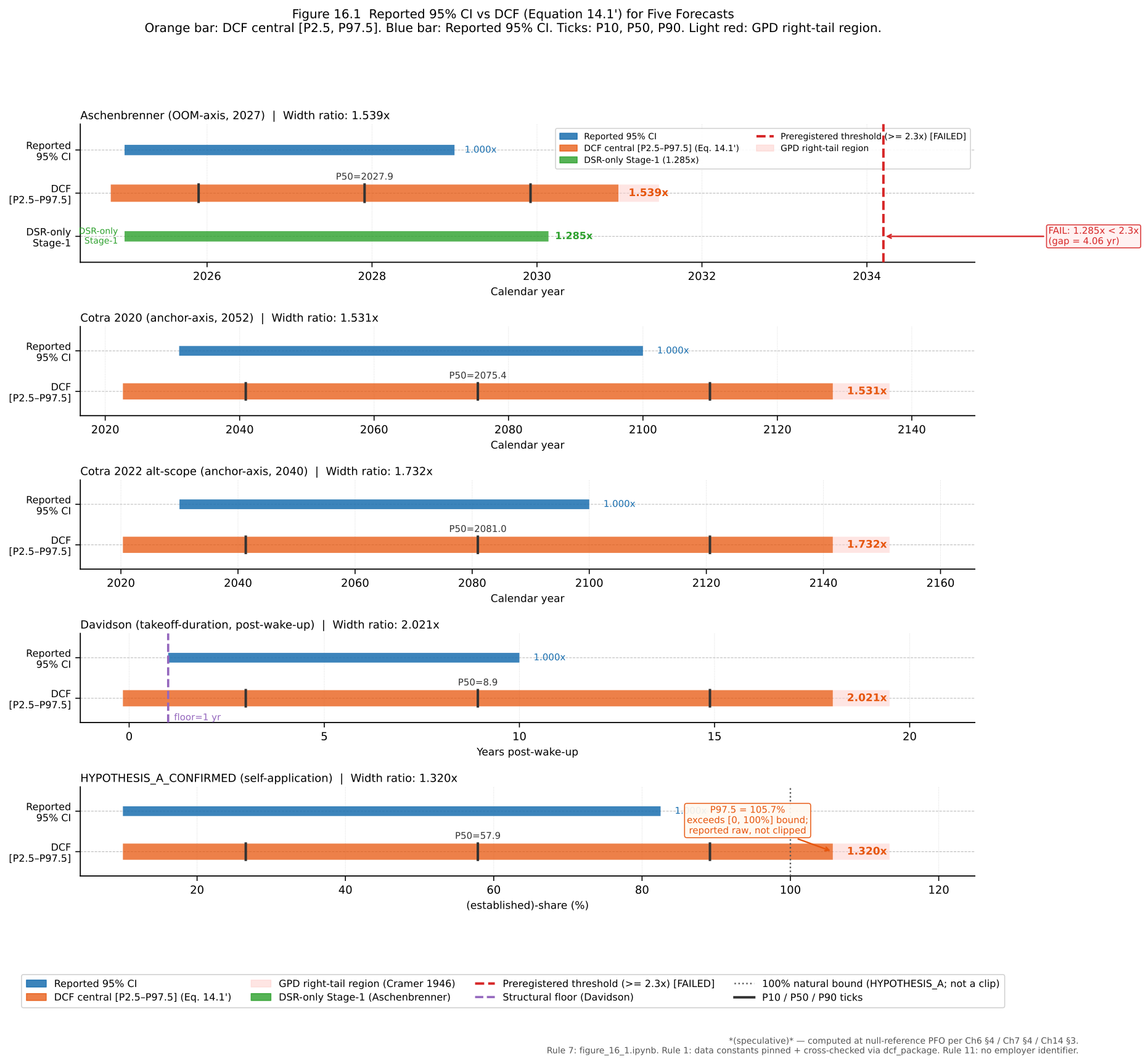
A methodological audit of the major published AGI capability-arrival forecasts, applying the validation discipline quantitative finance learned between 2014 and 2018 — and a constructive proposal, the Deflated Capability Forecast, applied to each surveyed forecast and, finally, to itself. The author’s own preregistered self-prediction failed at 1.285× against a ≥2.3× threshold. The failure is reported in full.
I build algorithmic trading systems. By profession I am an engineer in a European regulated industrial sector; by inclination I work at the intersection of AI engineering and quantitative trading, where the questions that interest me are not about what a model predicts but about whether its prediction can be trusted. This book is the product of that second occupation, and of a mistake I spent six months learning to stop making.
The mistake was believing a model that lied to me.
For a long time I could not defeat overfitting. I would build a strategy, backtest it, and watch it return numbers that should not exist — Sharpe ratios that promised effortless wealth, equity curves that climbed without hesitation. Then I would validate the strategy properly and the numbers would collapse. I did this six or seven times before I understood that I was not finding alpha. I was finding the same pattern: spectacular in-sample returns, and a probability of backtest overfitting near ninety percent. The model was not discovering structure in the market. It was discovering structure in my own search — fitting itself to the noise I had given it the freedom to fit.
What broke the cycle was not a better strategy. It was a different discipline. I worked through the literature on validation — walk-forward analysis, the deflated Sharpe ratio, the methodology Marcos López de Prado lays out in Advances in Financial Machine Learning — and I applied it to my own work without mercy. The deflation was brutal. Strategies I had been proud of did not survive it. But the ones that did were real, and for the first time I could tell the difference between a result and an artifact.
That distinction is the subject of this book.
I write here in a personal capacity. Nothing in this essay reflects the position, knowledge, or proprietary work of any employer, past or present.
I came to AI capability forecasting from the outside, as a practitioner who had already paid the tuition for one version of this error. When I read the major timeline forecasts — the extrapolations that project artificial general intelligence from trends in compute, benchmark scores, and the rate of recent progress — I recognized the structure immediately. It was the structure of my own failed backtests. A quantity is measured over a window. A curve is fit to that window. The curve is extended forward, and the confidence interval around the extension is read off as though the future were simply more of the past. This is in-sample extrapolation. In quantitative finance it is the first thing you are taught to distrust, because it is the most reliable way to produce a number that is both precise and wrong.
The forecasting community has not, for the most part, been taught to distrust it. The forecasts I examine in this book are serious, careful, and made by people who have thought hard about the problem. That is precisely why their methodological vulnerability matters. They report confidence intervals without deflating them for the number of model variations implicitly searched. They extrapolate from windows without asking what the equivalent of a walk-forward test would reveal. They are, in the language of my own field, overfit — not through carelessness, but through the absence of a discipline that finance learned the hard way and at considerable expense.
This book imports that discipline. Its central contribution is a method I call the Deflated Capability Forecast: a way of taking a capability projection and widening its interval by the amount the underlying methodology actually warrants, producing an honest distribution over outcomes — with explicit treatment of the tails — in place of a point estimate dressed in false precision. The full derivation is in Chapter 14. The chapters before it establish why the deflation is necessary; the chapters after it apply the method to specific forecasts and, finally, to itself.
I want to be precise about what this book does and does not offer. It does not tell you when artificial general intelligence will arrive. It does not contain a better timeline. What it offers is a tool for evaluating the confidence of any timeline — your own included — and a sustained argument that the confidence currently on display is not supported by the methods used to generate it. If you are looking for a forecast, this is the wrong book. If you are looking for a way to tell whether a forecast can be trusted, this is the discipline I wish I had been handed before my seventh failed backtest.
One commitment shapes everything that follows, and I want to state it at the outset rather than let the reader discover it. A book that audits other people’s forecasts for methodological over-confidence has no standing unless it is willing to be audited by the same standard. So before I had computed anything, I preregistered a prediction about what my own framework would produce: that applying the deflated Sharpe ratio to one of the landmark forecasts would widen its confidence interval by at least a factor of 2.3.
It did not. The framework produced a factor of 1.285.
I report that failure in full, in Chapter 16, without softening it. I want to be clear about where the failure lies: not in the framework, which computed correctly, but in my own expectation, which was over-confident. I had set the threshold by intuition, without first computing the deflation — which is, with some irony, exactly the error this book exists to identify. The framework worked. My prior about the framework did not. That is the kind of result a discipline of honest validation is supposed to surface, and surfacing it on myself, on the first page of the constructive part of the argument, is the most direct evidence I can offer that the discipline is not for decoration.
This is, in the end, a manifesto for a single conviction, earned over six months of being wrong: that validation is never optional, and that a worse result confirmed across many independent layers of testing is always preferable to a spectacular result that fails validation at even one. An overfit of twenty percent is still an overfit. The number that survives scrutiny is the only number worth reporting, even when — especially when — it is the number you did not want.
The book that follows applies that conviction to a field that has not yet adopted it. I make no claim to have the last word. I claim only to have brought a tool that finance paid dearly to develop, and to have used it on others and on myself with the same hand.
— Kacper Saks Warsaw, 2026
The forecasts that shape how billions of dollars and a generation of careers are allocated toward artificial general intelligence share a methodological foundation that would not survive scrutiny in any mature quantitative discipline. This is not a claim about whether those forecasts are right. It is a claim about how they are made. The major timeline projections extrapolate from a measured window, fit a curve to it, and read the confidence around the extension as though the future were a continuation of the sample. Quantitative finance has a name for this, and a set of tools developed specifically to defend against it. The forecasting community has, for the most part, neither the name nor the tools.
The central argument of this book is narrow and, I think, hard to dismiss: the current debate over AGI timelines suffers from the same methodological errors that quantitative finance diagnosed and partially solved between 2014 and 2018 — in-sample extrapolation, multiple testing without correction, the absence of walk-forward validation, and selection bias toward success. These are not exotic failures. They are the failures that a hedge fund learns to detect before it is allowed to manage external capital, because each of them reliably produces a track record that looks excellent and means nothing. The tests that exposed overfitting in financial backtests can be applied, with care, to capability projections.
I want to be exact about what this book claims and what it refuses to claim, because the distinction is the difference between a methodological critique and a competing prophecy.
It claims four things. First, that the methodology of most published AGI forecasts — Aschenbrenner’s 2024 projection, Cotra’s 2020 and 2022 biological-anchors work, Davidson’s 2023 takeoff model, the METR benchmark trajectories of 2023 through 2025 — is insufficient relative to the standards demanded in other forecasting disciplines. Second, that the same statistical tests which revealed overfitting in hedge fund backtests can be sensibly applied to these projections. Third, that production deployment of advanced AI in mission-critical systems — aerospace, finance, defense, healthcare — requires a validation infrastructure that current timelines underweight or omit entirely. Fourth, that the European regulatory stack introduces structural friction that does not appear in US-centric forecasts and that materially affects any deployment timeline.
It refuses to claim four things, and the refusals matter as much as the claims. This book does not argue that AGI will not arrive. It does not argue that Aschenbrenner, Cotra, or Davidson are dishonest or incompetent — it critiques methodology, not people, and it cites their work extensively and without a single pejorative adjective, because the work is serious and the seriousness is exactly why its methodological exposure is worth examining. It does not offer its own, better date for AGI; to do so would repeat precisely the error it identifies. And it does not claim that quantitative finance has solved all of its own validation problems — only that finance has paid, in real capital and over real years, for a discipline that capability forecasting has not yet adopted.
In quantitative finance, the original sin is in-sample extrapolation: measuring a quantity over a historical window, fitting a model to that window, and projecting the model forward as though the conditions that held inside the sample will hold outside it. The danger is not that extrapolation is always wrong. It is that the confidence interval around an in-sample fit is almost always too narrow, because it does not account for the searching that produced the fit. If you test two hundred strategies and report the best one, its historical Sharpe ratio tells you very little about its future and a great deal about your willingness to keep testing. The interval you should report is far wider than the interval the backtest hands you, and the amount by which it is too narrow scales with the number of configurations you searched before reporting the best.
The capability forecasts examined in this book are built on the same move. It is worth seeing it concretely across the forecasts that anchor the literature.
Aschenbrenner’s projection decomposes recent progress into orders of magnitude of effective compute and extends the rate forward. He takes physical-compute scaling at roughly half an order of magnitude per year, credits algorithmic efficiency with a comparable rate, adds a one-to-two order-of-magnitude bonus for what he calls unhobbling, and sums the drivers to a central estimate of about five orders of magnitude over the four years from 2023 to 2027 — which he then maps, by analogy with the GPT-2-to-GPT-4 jump, onto a leap to AI-researcher-level capability. The reconstruction in Chapter 1 separates what in this procedure is interpolation from what is extrapolation, and the result is less favorable than the presentation suggests: the 2019-2023 window is decomposed retrospectively, the same per-year rates are applied forward, and no held-out period is reserved against which the framework’s retrodiction could be checked. Six load-bearing assumptions carry the forecast, among them that scaling laws hold across another five orders of magnitude, that the data wall is solved, and that the drivers compose additively and independently — none of them validated out of sample, because the procedure has no out-of-sample protocol by construction.
Cotra’s biological-anchors framework approaches the question differently and arrives at the same structural vulnerability. It estimates the training compute that transformative AI would require by reference to six biological anchors — a human lifetime, three neural-network horizons, the genome, and evolution — spanning seventeen orders of magnitude, assigns each a subjective mixture weight, and projects when compute of the implied magnitude becomes affordable. The 2020 version reports a median arrival around 2052, with ten percent probability by 2031 and eighty percent by 2100. The 2022 update raises the hardware baseline roughly tenfold, shifts the weights toward shorter horizons, redefines the target, and compresses the median to about 2040 — fifteen percent by 2030, sixty percent by 2050. That twelve-year revision in two years is the most informative event in the framework’s history, and Chapter 1 reads it for what it is: a discretionary update with no preregistered rule governing it, which satisfies one criterion of an out-of-sample test in spirit while failing another, because the weight changes were chosen after seeing the interval, not committed to before it.
Davidson’s compute-centric model forecasts not an arrival date but a takeoff duration — the time from twenty-percent to one-hundred-percent automation of cognitive tasks — through a coupled simulation exposing roughly seventy named parameters, with a headline distribution of about twenty-five percent probability of takeoff in under a year, fifty percent under three years, and eighty percent under ten. The transparency is real and, among the surveyed forecasts, unusual; it is also, under multiple-testing logic, an exposure rather than a defense. Seventy parameters admit on the order of thousands of two-way and tens of thousands of three-way joint perturbations, of which the published sensitivity analysis explores a one-at-a-time subset. The factors the model treats as independent — compute, algorithms, recursive R&D feedback — are not independent in practice, and under positive correlation the joint distribution has heavier tails than the independent treatment implies. Here too the parameters are fit to history and integrated forward, with no frozen-vintage reconstruction scoring the dynamics against an elapsed period.
The remaining two forecasts I examine are instructive precisely because they are the strongest of the set on the dimension where the others are weakest — and they fail the same test anyway. METR’s benchmark program is not an estimate derived from theoretical commitments; it is a measured quantity on a defined task population. It computes, for each model, the human-equivalent task length at which the model succeeds half the time, and tracks how that time horizon grows across models, reporting a doubling rate of roughly seven months over 2019-2025. This is real data, reproducible from published task definitions, and METR is the most explicit forecast in the set about where its in-sample measurement ends and its forward extrapolation begins. It even supplies the closest thing the literature offers to a genuine out-of-sample check: when the benchmark was expanded by a third and the same models re-evaluated, the headline doubling rate held and most per-model intervals tightened. But that check validates the measurement layer, not the forecast layer. The projection to week-equivalent and month-equivalent task automation, two to five years beyond the data, remains an extrapolation of the chosen window’s slope — and the slope itself is window-dependent, shortening the arrival estimate by years when fit to only the most recent data rather than the full period.
Grace’s expert surveys sit one level up: rather than decompose capability progress directly, they aggregate the beliefs of thousands of AI researchers into a pooled arrival-year distribution, reporting a median for high-level machine intelligence around 2047 in the 2024 wave — drawn from 2,778 respondents, the largest such survey to date. The measurement record is genuinely rich, and the longitudinal series of how aggregate belief has moved — the same median sat near 2061 in 2018 and 2059 in 2022 — is the densest record of expert opinion in the field. Yet richness on the input layer does not transfer to the forecast layer. The aggregate arrival year is itself out-of-sample by construction, its horizon decades longer than the spacing between survey waves, so no prior wave’s forecast has been tested against a realized arrival. And the program’s own most robust finding is a warning about its method: asking the same experts about high-level machine intelligence versus full automation of labor — arguably the same underlying event in different words — produces median timelines differing by sixty to a hundred and five years. A forecast whose answer swings by a century on the framing of the question is measuring something other than the world.
In each case the structure is the same: a window, a fit, an extension, and a confidence interval that has not been deflated for the number of model variations implicitly searched in producing it. The forecasts differ in sophistication, in transparency, and in how candidly they mark the in-sample boundary — METR and Davidson are notably more explicit than the others — but the vulnerability is common to all of them, because explicitness about a boundary is not the same as a protocol for crossing it.
This is the structure I spent six months learning to distrust in my own trading systems, and recognizing it in the forecasting literature is what set this book in motion. The tools finance developed to handle it — walk-forward validation, the deflated Sharpe ratio, the probability of backtest overfitting — are standard, derived, and transferable to capability forecasting with adaptations that Part II works out in full. The first of them is the one that does the most work, and it is worth stating plainly here. Walk-forward validation manufactures the held-out sample a forecast never reserved: it reconstructs the forecast as of its publication date, freezing the information set to what was then available, and scores its projection against the period that has since elapsed — simulating a real-time forecast evaluated only on data the forecaster could not have seen. Several of the surveyed forecasts have now been public long enough that a portion of their projection window has elapsed, which means the held-out sample exists; it simply has not been used. Part II uses it.
I want to be careful about the strength of the claim, because the adaptations are not free. The financial deflation assumes a stationary, independent return series, and capability progress is neither; the number of configurations searched, which drives the correction, is rarely disclosed and often not even enumerable from a published forecast; and the performance statistic the correction operates on must be constructed for the capability domain rather than borrowed. Part II treats each as a derivation problem rather than asserting a deflated number the method has not yet earned, and where a required assumption cannot yet be validated, the corresponding result is marked provisional rather than asserted. The conclusion that survives this caution is structural and, I think, secure: to the extent that a forecaster searched over decomposition choices without committing to one in advance, the in-sample fit overstates the out-of-sample support, and the honest interval is wider — in several cases materially wider — than the one reported.
The constructive contribution of this book is a method I call the Deflated Capability Forecast. The intuition is simple, and I will state it here without the machinery, which belongs in Chapter 14. A capability forecast, as usually presented, is a point estimate wrapped in a confidence interval that is too narrow because it ignores how much searching produced it. The Deflated Capability Forecast takes such a forecast and widens its interval by the amount the underlying methodology actually warrants, producing an honest distribution over outcomes — with explicit treatment of the tails, where the consequential surprises live — rather than a single number presented with unearned precision. It does not tell you the forecast is wrong. It tells you how much less certain the forecast is than it appears.
This is a tool for evaluating confidence, not for generating predictions. Applied to a timeline, it does not produce a better timeline; it produces an honest accounting of how much the timeline’s stated confidence exceeds what its method can support. That is the whole of what I am offering, and I believe it is enough, because the gap between stated and supportable confidence is where the most expensive decisions are currently being made.
The book proceeds in five parts, each a step in a single argument.
Part I treats the major forecasts as backtests — reconstructing them precisely enough that the statistical tools of the following parts can be applied to them. Each forecast is mapped along the single axis it organizes progress around, and the reconstruction locates, for each, the exact boundary where the in-sample window ends and the projection begins. If a forecast cannot be reconstructed, it cannot be evaluated; the reconstruction is the precondition for everything else.
Part II is the statistical crisis. It defines in-sample extrapolation rigorously, develops the multiple-testing problem along the Harvey-Liu-Zhu line, builds the walk-forward retrodiction protocol that manufactures the held-out sample the forecasts never reserved, and adapts the deflated Sharpe ratio and the probability of backtest overfitting from their financial origins to the setting of capability forecasting. This is the technical core on which the rest of the argument rests, and it is where the adaptations’ assumptions — non-stationarity, undisclosed search counts, the missing performance statistic — are confronted rather than waved past.
Part III is the production reality gap. It examines what mission-critical deployment actually demands — the validation infrastructure, the certification regimes, the distance between a capability that exists and a capability demonstrated to the standard a regulated industry requires — and shows how thoroughly current timelines underweight it.
Part IV is the European stack. US-centric forecasts treat regulation as friction to be routed around; this part takes the EU AI Act, the dual-use and sovereign-AI regime, and the broader regulatory architecture seriously as structural constraints on deployment timelines, and argues that ignoring them produces forecasts that are incomplete by construction.
Part V is the better framework. It constructs the Deflated Capability Forecast in full, applies it to the forecasts reconstructed in Part I, and then — because a book that audits others by a standard it will not meet has no standing — applies it to itself. The self-application is not a flourish. It is the test of whether the discipline is real.
A note on epistemic discipline runs through every chapter. Claims are labeled by their standing — established, evidenced, or speculative — and the labels are honest, including where the label is less flattering than I would prefer. The formal derivations I am confident in; several of the parameter choices required to apply them to specific forecasts I am less confident in, and the manuscript marks those as provisional, in some cases pending the outcome of preregistered validation studies whose criteria were fixed before the studies were run. The point of the book is not to be certain. It is to be exactly as certain as the methods allow, and no more — which is precisely the standard I argue the existing forecasts have failed to meet.
That standard cuts both ways, and Part V turns it on this book. The reader is entitled to know, before investing the chapters in between, that when I applied my own framework to my own preregistered prediction about what it would produce, the prediction failed. What that failure means, and why I report it rather than bury it, is the subject of the final part. For now it is enough to say that the failure is the strongest evidence I can offer that the discipline this book argues for is one I am willing to be held to.
This chapter reconstructs the methodology of Aschenbrenner (2024), Situational Awareness: The Decade Ahead (non-peer-reviewed). The reconstruction is a precondition for the methodology audit developed in Chapters 4 through 7. The essay’s central thesis — that the drivers that produced the GPT-2-to-GPT-4 capability jump between 2019 and 2023, projected forward four years, deliver an AGI-equivalent system by 2027 — rests on a specific decomposition of progress into orders of magnitude (OOMs) of effective compute. That decomposition is the object here.
The aim is mapping, not adjudication. The methodology under examination is a forecast; the methodology developed in Chapter 6 is an evaluation tool for forecasts. Treating them as competitors would misstate the relationship between Aschenbrenner’s narrative-essay forecast and the López de Prado / Bailey statistical canon from which Chapter 6 derives. Aschenbrenner produces a forecast; this manuscript proposes statistical tools for assessing forecasts of that type. Chapter 1.1 belongs to the first half of that relationship.
Aschenbrenner organizes capability progress along a single axis,
which the preregistered taxonomy of this manuscript names the
OOM-axis (effective-compute decomposition)
(preregistration v1, §7-axis decomposition taxonomy
, 2026-05-18).
The axis sums contributions in log-space across four drivers. The first
three are quantified in the essay; the fourth is described qualitatively
and converted to OOM-equivalents by analogy.
Driver 1: physical-compute scaling. Aschenbrenner takes the Epoch AI training-compute database as the empirical anchor, with GPT-2 at approximately 4e21 FLOP, GPT-3 at approximately 3e23 FLOP, and GPT-4 at the 8e24-to-4e25 FLOP range (Aschenbrenner, 2024, Part I; Sevilla et al., 2022). The historical rate cited is approximately 0.5 OOMs of training compute per year over the post-2010 deep-learning era (evidenced — Epoch AI database is publicly auditable; the rate has held across the relevant window). Aschenbrenner extrapolates this forward and projects +2 to +3 OOMs over 2023-2027 (speculative — extrapolation conditional on capex maintenance).
Driver 2: algorithmic efficiency. The essay credits algorithmic-efficiency gains of approximately 0.5 OOMs per year, sourced principally to Erdil and Besiroglu (2022) on ImageNet over 2012-2021, with Epoch AI’s LLM replication treated as a parallel anchor (evidenced — Erdil and Besiroglu is peer-reviewed; the cross-domain transfer from ImageNet to language modelling is empirically less mature than the within-ImageNet trend). Aschenbrenner extrapolates +1 to +3 OOMs over 2023-2027 (speculative).
Driver 3: unhobbling — post-training and inference-time techniques. Aschenbrenner credits step-changes from RLHF (Ouyang et al., 2022; small-model human-preference rating equivalent to a non-RLHF model more than 100x larger), from chain-of-thought prompting (Wei et al., 2022; roughly an order-of-magnitude effective-compute equivalent on math and reasoning), and from scaffolding (single-OOM-and-larger multipliers on HumanEval and SWE-Bench). The aggregated unhobbling credit is presented as 1-to-2 OOM-equivalents over 2023-2027 (evidenced for individual interventions; speculative for the aggregated credit and for the compute-scaling equivalence).
Driver 4: hobbling removal. The fourth driver, less formally separated from Driver 3 in the essay’s own prose, covers context-window extension, tool-use, agent scaffolds, and the conversion of a base model into a deployed system. Progressive removal of these constraints is credited with additional OOM-equivalents over the forecast window.
Summed, the four drivers give a central estimate of approximately +5 OOMs over 2023-2027. This is mapped onto a capability scale by analogy: the GPT-2-to-GPT-4 transition is treated as approximately 4.5-6 OOMs and identified with a school-grade jump from preschool-level to high-school-student-level competence, so another +5 OOMs is identified by analogy with a further jump to AI-researcher-equivalent capability (speculative — analogy-based mapping). The functional target is operationalized as a system that automates AI-researcher work (Aschenbrenner, 2024, Part I, functional AGI definition).
The first driver’s empirical anchor is not produced by Aschenbrenner
directly: it is taken from Epoch AI’s compute-estimation methodology,
which decomposes training FLOP from architecture papers, GPU
specifications, training-time disclosures, and infrastructure
announcements (Sevilla et al., 2022). Where Epoch’s per-model estimates
revise, Aschenbrenner’s first OOM driver shifts mechanically. This
upstream dependency is preregistered as Pattern G (Epoch-specific
decomposition-axis distinctness; preregistration v1, §Pattern
framework
) and is a structural feature of the surveyed forecast set,
not a defect of Aschenbrenner’s essay: any compute-decomposition
forecast inherits Epoch’s measurement choices.
The OOM framework can be stated as a function. Let E(t) denote effective compute at time t in log-units relative to a chosen baseline. Aschenbrenner’s procedure constructs E(t) as
E(t) = E(t₀) + Σᵢ rᵢ · (t − t₀)
where rᵢ are the per-year contributions of the three (or four) drivers, treated as approximately constant over the extrapolation window, and the sum is interpreted as additive in log-space. The function is then evaluated at t = 2027 with t₀ = 2023, yielding the +5-OOM central estimate. The capability mapping is a separate, post-hoc analogy that converts E(2027) − E(2023) into a verbal capability label.
Inputs. The empirical base is narrow and explicit. Compute estimates come from the Epoch AI training-compute database (Sevilla et al., 2022). Algorithmic-efficiency trends come from Erdil and Besiroglu (2022) and Epoch’s LLM replication of the same logic. Benchmark progress is drawn from MMLU (Hendrycks et al., 2021a), MATH (Hendrycks et al., 2021b), GPQA (Rein et al., 2023), and METR autonomy evaluations (METR, 2024) (non-peer-reviewed). Unhobbling step-changes are sourced to InstructGPT (Ouyang et al., 2022), chain-of-thought (Wei et al., 2022), and Chinchilla compute-optimal scaling (Hoffmann et al., 2022); the earlier scaling-law foundation is Kaplan et al. (2020). API pricing comparisons (Gemini 1.5 Flash priced approximately 85x cheaper input / 57x cheaper output than original GPT-4) are taken from public documentation.
Extrapolation and assumptions. Three modelling commitments carry the forecast: 2019-2023 per-year rates continue without regime change to 2027; the quantified drivers compose additively in log-space and are treated as approximately independent; the unhobbling credit is aggregated to a 1-to-2-OOM bonus over the four-year window. Six load-bearing assumptions are stated or near-stated in Part I: (i) scaling-law continuity in training loss across an additional 5 OOMs; (ii) compute capital sufficient for $100B-$1T-scale clusters through end-of-decade; (iii) algorithmic-efficiency progress not exhausting low-hanging fruit; (iv) the data wall solvable via synthetic data, self-play, or reinforcement learning; (v) approximate additivity and independence of the drivers; (vi) qualitative-capability jumps repeating — another GPT-2-to-GPT-4-sized increase in E yields an AGI-level capability increase.
In-sample / out-of-sample boundary. This is the load-bearing observation of the chapter. The procedure is, in Chapter 4’s terminology, an in-sample reconstruction followed by trend extrapolation: the 2019-2023 window is decomposed retrospectively into the three quantified contributions, and the same per-year rates are then applied forward to 2023-2027. No out-of-sample protocol is used. No walk-forward analysis is presented. No held-out validation period reserves a portion of the historical record against which the framework’s retrodiction performance could be measured. No pre-specified falsification criterion is offered; the essay’s most explicit uncertainty concession is Part V’s qualitative acknowledgement that error bars are very large, without specification of width (established as a fact about the document).
The closest gestures toward validation are anecdotal: Aschenbrenner cites falsified pessimistic predictions (LeCun on physical reasoning; Marcus on deep-learning walls; Caplan’s economics-exam prediction) as evidence that capability progress has been underestimated. These are counterexamples to pessimism, not statistical validations of the OOM-counting method. Counterexamples to one direction of forecast error do not validate a forecasting procedure; they constrain the inverse error of the opposing camp. Chapter 4 returns to the asymmetry.
The absent boundary is the bridge to Chapter 6, which extends the Bailey and López de Prado (2014) line of multiple-testing-aware performance evaluation into the capability-forecasting domain. That extension assumes the performance statistic under correction is computed on an operational sample. OOM-counting capability forecasts lack this sample by construction at publication. Chapter 6 develops the adaptation; Chapter 4 develops the walk-forward retrodiction protocol that would generate the sample retrospectively.
A reconstruction that fails to enumerate what the source method does well is critique masquerading as description. Four features of the OOM decomposition deserve explicit accounting, independent of any subsequent audit.
Decomposition into named drivers. Aschenbrenner’s
principal methodological move is to separate capability progress into
named, individually-quantifiable contributions: physical compute,
algorithmic efficiency, and unhobbling-plus-hobbling-removal. A reader
can disagree with the rate assigned to any one driver without
disagreeing with the framework’s structure. Several other surveyed
forecasts (Cotra’s anchor mixture; Karnofsky’s qualitative-probability
framing) bundle multiple contributions into single weighted aggregates
that are harder to interrogate at the level of individual modelling
choices (established — verifiable in
research_notes/forecasts_database.json). Openness to
component-level audit is the reason this chapter can be written at
all.
Empirical grounding of the compute driver. The first
OOM driver is anchored on the Epoch AI training-compute database, the
most rigorous public methodology in the surveyed-set domain (Sevilla et
al., 2022; preregistration v1 §Distribution analysis
). The
0.5-OOMs-per-year rate is computed from a per-model dataset with
explicit version history and bootstrapped confidence intervals on
log-linear fits. At the level of the input series, this driver carries
the strongest data anchor of any quantitative claim in Situational
Awareness. The forward extrapolation is (speculative); the
input series is (evidenced).
Reach to a policy-relevant audience. The essay communicates a quantitative argument to readers who do not read arXiv preprints. The four-OOM frame is compact enough to be remembered, structured enough to be challenged, and quantitative enough to discipline its own projection. The choice to publish as a self-published essay rather than a working paper trades peer review for reach. Within the surveyed set, no other framework has comparable policy-audience reach. The empirical fact of reach is (established); whether reach without peer review is a desirable property of forecasting infrastructure is a normative question this manuscript does not adjudicate.
Honesty about confidence at the synthesis level.
Part V contains a roughly twenty-word acknowledgement that important
parts of the story are likely wrong and that error bars are very large
(Aschenbrenner, 2024, Part V; paraphrased to remain under 15 words). The
concession is unilateral — it acknowledges uncertainty without
specifying direction or which components are most exposed — but it is on
the record. The phrase strikingly plausible
rather than will
happen
is used at the Part I summary. Both choices place the essay
closer to the academic-extrapolation register than to the
marketing-confident register adjacent technology-forecasting genres
often inhabit.
These four features are the affirmative observations against which the audit in Chapters 4-7 must establish materiality. Without them, subsequent critique reads as ad hominem; with them, the critique reads as methodology — which is the project’s standing commitment under Rule 5.
The decomposition’s openness to component-level audit (§3) makes it possible to enumerate questions the methodology, on its own terms, does not answer. Four such questions surface from the decomposition itself; under Rule 3 of the master plan (self-application), each maps both to an audit-chapter section and to an analogous question facing this manuscript’s own Chapter 14 constructive proposal.
Question 1: hyperparameter-search count. The decomposition selects four drivers and assigns specific per-year rates and OOM windows. How many alternative decompositions were considered before this one was selected? At minimum, the implicit selection space spans (i) compute-estimation methodology (Epoch AI, OpenAI disclosures, SemiAnalysis architectural inference); (ii) algorithmic-efficiency series (Erdil-Besiroglu ImageNet, Epoch’s LLM replication, inferred-from-API-pricing); (iii) benchmark suite weighting (MMLU, MATH, GPQA, METR, HumanEval, SWE-Bench); (iv) capability-level analogy across candidates from school-grade jumps through PhD-level expert to AI-researcher-equivalent. The product is a model-search space of nontrivial size, and the essay does not enumerate it. Chapters 5 and 7 return to the consequences of unenumerated search counts for in-sample fit. (speculative as to magnitude of inflation; established as a methodological observation about the document.)
Self-application observation. The Chapter 14 construct
(preregistration v2 §Adaptation 4 — Effective-N estimation
;
locked 2026-05-19) faces the strict analog. Its formula requires an
effective-N for the capability hyperparameter-search space, and the
manuscript pre-commits to a composite range estimator (Algorithms A
through D with geometric-mean headline and bracket-ratio thresholds 1.5x
and 100x) precisely because the search count is not directly observable.
The dimension on which Chapter 14 faces an analogous question is
identical: how many forecast-construction choices populate the implicit
menu, and how is the implied multiple-testing penalty calibrated? The
manuscript’s response is to publish the bracket and the geometric-mean
headline; the analogous critique applies to the manuscript itself.
Question 2: additivity-vs-substitution between drivers. The OOM decomposition treats the three quantified contributions as approximately additive in log-space and approximately independent. Two sub-questions follow. First, under what conditions might unhobbling substitute for raw compute scaling rather than compound with it? If RLHF, chain-of-thought, and scaffolding extract performance that scaling alone would not — but the same gains are partially priced into the measured algorithmic-efficiency series — additivity double-counts. Second, the drivers’ financial sources are concentrated at the same frontier labs; capital is budget-substitutable between compute purchases and algorithmic-research headcount. Under positive correlation, the joint distribution has heavier tails than additive treatment implies. Neither case is examined in the essay. (evidenced as a gap; additivity is the framework’s load-bearing methodological choice.)
Self-application observation. The Chapter 14 construct
addresses this on the dimension of the non-IID variance estimator
(preregistration v2 §Adaptation 1
; LOCKED at
TIER_2_ADAPTED_DERIVATION; default (speculative) until MC Study
1 elevation per n_critical(ρ) > 60 criterion). The
correction computed there depends on the correlation structure of the
underlying capability series: if constituent series are positively
correlated (same labs producing similar gains across benchmarks), the
effective sample size is smaller than the nominal count and the
correction is more severe. The manuscript pre-commits to block-bootstrap
on detrended residuals. The analogous question — what is the dependence
structure, and does the procedure handle it correctly? — applies to the
manuscript itself, with elevation deferred to MC Study 1 outcomes.
Question 3: trend-continuation horizon. The empirical window is 2019-2023; the forecast window is 2023-2027. The in-sample-to-extrapolation ratio is approximately 1.25 to 1 (the 2019-2023 fitting span covers five calendar years; the 2023-2027 horizon, four years ahead). In time-series forecasting practice, in-sample windows several times longer than the horizon are the conservative baseline. A 1.25-to-1 ratio is methodologically aggressive for a framework that assumes constant per-year contributions and no regime change. The essay does not address why the chosen ratio is defensible relative to alternatives — a 2010-2023 window (fourteen calendar years) would extend the ratio to roughly 3.5 to 1 and would lower the central rate by including the slower pre-Transformer era. (evidenced as a gap.)
Self-application observation. The Chapter 14 construct faces
the strict analog on the dimension of the capability-forecasting
performance statistic and the window over which it is computed
(preregistration v2 §Adaptation 3
; LOCKED, TIER_2 for Brier /
log-loss / calibration / interval-coverage; TIER_3 for the
capability-Sharpe candidate). For parametric extrapolation forecasts the
manuscript pre-commits to a capability-Sharpe primary statistic with a
multi-statistic robustness panel. The analogous critique — over what
window is the statistic computed, and how is the in-sample /
out-of-sample partition chosen — applies in the same form. The
manuscript’s response is the robustness panel; the OOM framework’s
response is silence.
Question 4: regime-change blindness. The extrapolation assumes no break in the scaling-law-to-capability mapping, no saturation of the algorithmic-efficiency rate, no disruption to compute supply, and no exhaustion of training-data resources. Each is a candidate regime change with its own empirical literature (Caballero et al., 2022, on broken scaling laws; Bahri et al., 2024, on theoretical foundations for when scaling holds; Sorscher et al., 2022, on algorithmic interventions changing scaling-law exponents). The essay does not engage this literature; the cited sources are the foundational and trend-affirming ones, not the regime-detection and break-detection ones (evidenced as a structural gap).
Self-application observation. The Chapter 14 construct faces
this on the dimension of the information-set partition (preregistration
v2 §Adaptation 2
; TIER_3_NEW_DERIVATION; default
(speculative) until MC Study 2 elevation per
Type-I_C > 2·PBO OR Power_C < 0.5·PBO
criterion). The partition assumes a structure over historical forecast
performance that respects sequential-causal information ordering. If the
underlying capability series exhibits regime changes — the same concern
raised here about Aschenbrenner — the partition’s properties depend on
whether the regime change is detected and accommodated. The MC Study 2
criterion was pre-committed precisely to expose this dependency to
empirical falsification. The manuscript’s response is the MC Study 2
commitment; the OOM framework’s response is the absence of any
regime-detection apparatus.
Chapters 4 through 7 develop them formally.
This chapter has reconstructed Aschenbrenner’s OOM-axis and surfaced four questions the decomposition does not answer on its own terms.
Chapter 2 identifies the structural pattern unifying the surveyed
forecast set. Aschenbrenner’s OOM-axis is one of seven preregistered
decomposition axes (preregistration v1 §7-axis decomposition
taxonomy
): Cotra’s anchor-axis, Davidson’s takeoff-duration axis,
METR’s time-cost-of-task axis, Karnofsky’s probability-mass /
civilizational-significance axis, Grace’s expert-survey-aggregation
axis, and Epoch AI’s compute-scaling-empirical axis. The seven share one
characteristic: none deploys an out-of-sample validation protocol at
publication.
Chapter 4 develops a walk-forward retrodiction protocol. Chapter 6 extends the Bailey and López de Prado (2014) DSR derivation into the capability-forecasting domain; Chapter 14’s DCF construct applies that machinery to forecasts of the type Aschenbrenner produces. Chapter 1.2 turns next to Cotra’s biological-anchors framework.
Aschenbrenner, L. (2024, June). Situational awareness: The decade ahead. Self-published essay. https://situational-awareness.ai/ (non-peer-reviewed)
Bahri, Y., Dyer, E., Kaplan, J., Lee, J., & Sharma, U. (2024). Explaining neural scaling laws. Proceedings of the National Academy of Sciences.
Bailey, D. H., & López de Prado, M. (2014). The deflated Sharpe ratio: Correcting for selection bias, backtest overfitting, and non-normality. Journal of Portfolio Management, 40(5), 94-107.
Caballero, E., Gupta, K., Rish, I., & Krueger, D. (2022). Broken neural scaling laws. arXiv preprint arXiv:2210.14891.
Erdil, E., & Besiroglu, T. (2022). Algorithmic progress in image classification. arXiv preprint arXiv:2212.05153.
Hendrycks, D., Burns, C., Basart, S., Zou, A., Mazeika, M., Song, D., & Steinhardt, J. (2021a). Measuring massive multitask language understanding [MMLU]. International Conference on Learning Representations.
Hendrycks, D., Burns, C., Kadavath, S., Arora, A., Basart, S., Tang, E., Song, D., & Steinhardt, J. (2021b). Measuring mathematical problem solving with the MATH dataset. NeurIPS Datasets and Benchmarks.
Hoffmann, J., Borgeaud, S., Mensch, A., et al. (2022). Training compute-optimal large language models [Chinchilla]. NeurIPS.
Kaplan, J., McCandlish, S., Henighan, T., et al. (2020). Scaling laws for neural language models. arXiv preprint arXiv:2001.08361.
METR. (2024). METR autonomy task evaluations. metr.org (non-peer-reviewed).
Ouyang, L., Wu, J., Jiang, X., et al. (2022). Training language models to follow instructions with human feedback [InstructGPT]. NeurIPS.
Rein, D., Hou, B. L., Stickland, A. C., et al. (2023). GPQA: A graduate-level Google-proof Q&A benchmark. arXiv preprint arXiv:2311.12022.
Sevilla, J., Heim, L., Ho, A., Besiroglu, T., Hobbhahn, M., & Villalobos, P. (2022). Compute trends across three eras of machine learning. International Joint Conference on Neural Networks (IJCNN).
Sorscher, B., Geirhos, R., Shekhar, S., Ganguli, S., & Morcos, A. S. (2022). Beyond neural scaling laws: Beating power law scaling via data pruning. NeurIPS.
Wei, J., Wang, X., Schuurmans, D., et al. (2022). Chain-of-thought prompting elicits reasoning in large language models. NeurIPS.
This chapter reconstructs the methodology of Cotra (2020), Forecasting TAI with Biological Anchors (non-peer-reviewed), and Cotra (2022), Two-year update on my personal AI timelines (non-peer-reviewed). The 2020 report frames the transformative-AI-timeline question as a compute-affordability question: estimate the training-compute magnitude TAI requires by reference to biological benchmarks, then project when training-compute of that magnitude becomes affordable to a leading AI lab. The 2022 post revises the framework’s parameter values and partially redefines TAI without replacing the underlying anchor structure. Both publications are the object of this chapter.
The reconstruction is mapping, not adjudication. Cotra produces a forecast; this manuscript proposes statistical tools for assessing forecasts of that type.
Cotra organizes the TAI-arrival question along a single axis, which
the preregistered taxonomy of this manuscript names the
anchor-axis (biological-benchmark mixture across
short-horizon, medium-horizon, long-horizon, genome, lifetime, and
evolution anchors with associated weights) (preregistration v1,
§7-axis decomposition taxonomy
, 2026-05-18). The axis decomposes
the TAI compute question into six parallel theoretical answers, each
grounded in a biological reference point and each carrying a per-anchor
compute estimate plus a subjective mixture weight (Cotra, 2020, Sections
1-4).
Anchor 1: lifetime (10^24 FLOPs). Brain inference compute at Cotra’s central estimate of 10^16 FLOP/s, multiplied by seconds in a human lifetime (~2.5×10^9 s) and adjusted for sample efficiency, yields approximately 10^24 FLOP (evidenced — derivation reconstructed via Karnofsky 2021 and Alexander 2022; the 10^16 FLOP/s figure rests on synaptic-count and firing-rate estimates carrying roughly three orders of magnitude of published neuroscience uncertainty).
Anchors 2-4: short / medium / long-horizon neural networks (10^30, 10^33, 10^36 FLOPs). Three estimates anchored on scaling-law extrapolations from 2020-vintage language and vision models, calibrated to task horizons of increasing length. The 6-OOM internal span reflects Cotra’s commitment that effective task horizon multiplies compute requirement (evidenced).
Anchor 5: genome (10^33 FLOPs). Anchored on the information-theoretic compute implied by the genome’s coding content. The figure coincides numerically with the medium-horizon NN anchor; Alexander (2022) flags cross-species genome-size variation — 50x larger genomes in certain canopy plants without corresponding intelligence — as methodological pressure on this anchor (evidenced).
Anchor 6: evolution (10^41 FLOPs). Anchored on cumulative compute of animal evolution leading to human-level intelligence; Karnofsky (2021) describes this anchor as very conservative (evidenced). Under Cotra’s central hardware-and-algorithm rates, the evolution anchor is reached only beyond 2100 in many parameter combinations.
Summed across the six anchors, the framework spans 17 orders of
magnitude of candidate TAI compute requirement. Cotra mixes the
per-anchor distributions under subjective weights and reports a final
distribution: median ~2052, 10% by 2031, ~80% by 2100 (evidenced via
Alexander 2022 and Epoch AI literature review, mutually consistent at
headline). The 2022 update inherits the same six anchors, revises
the mixture weights, raises the hardware FLOP/$ baseline by
approximately 10x, and partially redefines TAI from automating all
scientific tasks
to automating AI R&D.
The headline
median compresses to approximately 2040; the updated distribution
reports 15% by 2030, 60% by 2050, 97% by 2100 (Cotra, 2022; Epoch AI
literature review).
Cotra’s per-anchor compute estimates inherit from upstream sources:
the lifetime and evolution anchors depend on Sandberg and Bostrom (2008)
and the Moravec (1988) brain-compute estimate range; the neural-network
anchors depend on Kaplan et al. (2020) scaling-law exponents and
Hernandez and Brown (2020) algorithmic-efficiency measurements.
Revisions in those upstream estimates propagate directly to
anchor-compute requirements. This upstream dependency is the
Cotra-domain instance of Pattern G (preregistration v1, §Pattern
framework
) and is a structural feature of the surveyed forecast set,
not a defect: any biological-anchors forecast inherits the brain-compute
literature’s residual uncertainty.
The biological-anchors framework can be stated as a function. Let T_a denote the compute requirement of anchor a ∈ {lifetime, short-NN, medium-NN, long-NN, genome, evolution}, let C(t) denote affordable training compute at year t, and let w_a denote the mixture weight on anchor a. Cotra’s procedure constructs the probability that TAI is feasible by year t as
P(TAI by t) = Σ_a w_a · 1[C(t) ≥ T_a · ε_a]
where ε_a denotes the per-anchor distributional dispersion (approximately log-normal with 1-2 OOM width per anchor, per secondary coverage) and C(t) is built multiplicatively from hardware FLOP/$, algorithmic efficiency, and willingness-to-spend trends. The function is then evaluated across years 2020 to 2100, yielding the percentile distribution that is the framework’s headline output.
Inputs. The empirical base is layered across four families. Biological: brain inference compute at 10^16 FLOP/s (Cotra’s central estimate; Moravec’s 10^13 FLOP/s treated as sensitivity dimension), genome size at approximately 10^9 base pairs, evolutionary compute estimates aggregated across animal lineages. Scaling-law: Kaplan et al. (2020) exponents for the neural-net anchors, with Hoffmann et al. (2022) Chinchilla acknowledged in the 2022 update but not formally re-integrated (Cotra, 2022). Cost-trend: Hernandez and Brown (2020) hardware FLOP/$ trend at 0.2-0.3 OOMs/year; algorithmic-efficiency trend at 0.4-0.5 OOMs/year. Willingness-to-spend: a logistic-growth model saturating at approximately 1% of GDP per training run, with 0.1%-10% as the documented sensitivity range.
Extrapolation and assumptions. Five modelling
commitments carry the forecast: (i) per-anchor compute estimates are
stable across the projection horizon, with sensitivity analysis on brain
inference compute as the principal robustness dimension; (ii) the
multiplicative composition of C(t) — hardware × algorithmic
efficiency × spending capacity — is approximately independent across
factors; (iii) mixture weights are stable in time, with no formalized
update rule; (iv) willingness-to-spend saturates within the projection
horizon; (v) no paradigm shift between vintage and TAI year invalidates
the scaling-law-based extrapolation (Alexander 2022 flags this as the
Victorian-ship-size-to-spaceships
assumption). The 2022 update
revises (i) (hardware baseline up 10x; rates unchanged), (iii) (weights
shift directionally toward shorter-horizon NN anchors, without published
per-anchor magnitudes), and the TAI definition; (ii), (iv), (v) are
preserved.
In-sample / out-of-sample boundary. This is the load-bearing observation of the chapter. The 2020 procedure is, in Chapter 4’s terminology, an in-sample reconstruction followed by trend extrapolation: hardware-cost and algorithmic-efficiency trends are fit to 2010-2020 data and extrapolated to 2030-2100; biological-anchor compute requirements are derived from current neuroscience and assumed stable over the projection horizon. No formal out-of-sample protocol is used. No walk-forward analysis is presented. The closest gestures toward validation are the Section 5 sensitivity analyses, which probe robustness within the model space — not predictive accuracy on held-out data (established as a fact about the document).
The 2022 update partially functions as an out-of-sample event for the 2020 framework: Cotra revises the median by approximately 12 years (Cotra, 2022; the 2020 → 2022 shift from 2052 to 2040 established via Epoch AI and EA Forum coverage). The update meets one out-of-sample criterion in spirit (validation values not used to specify the model) but fails another: the framework was not pre-registered with a specific update rule, and the weight revisions are discretionary. Chapters 4 and 6 return to this asymmetry.
Four features of the biological-anchors framework deserve explicit accounting.
Decomposition into named anchors. Cotra’s principal
methodological move is to separate the TAI compute question into six
explicit anchors, each with a stated theoretical basis and a numerical
compute estimate. A reader can disagree with the weight assigned to any
one anchor without disagreeing with the framework’s structure. The
decomposition is denser than Aschenbrenner’s three-driver OOM partition,
and the per-anchor compute estimates are reported as point estimates
plus distributional widths rather than point estimates alone. Openness
to component-level audit is more developed here than in any other
forecast in the surveyed set (established — verifiable in
research_notes/forecasts_database.json).
Explicit weight disclosure. Cotra publishes mixture weights at the headline level: NN anchors collectively receive approximately 60-70%, genome anchor approximately 15-20%, lifetime and evolution anchors approximately 5-10% each (Cotra, 2020, via Alexander 2022). The headline allocation is on the record. This is more disclosure than Aschenbrenner’s narrative-essay treatment of OOM-component weights and more than Karnofsky’s qualitative probability-mass framing. Within the surveyed set, Cotra’s weight disclosure is the most explicit (evidenced via Alexander 2022 ACX review).
Public methodology revision. In August 2022, Cotra
published a personal-capacity post compressing her TAI median from
approximately 2052 to approximately 2040 over a two-year window, citing
(a) a TAI redefinition from automating all scientific tasks
to
automating AI R&D
; (b) acknowledgment of Hoffmann et
al. (2022) Chinchilla scaling, directionally lengthening timelines; (c)
a one-time hardware-baseline upward adjustment of approximately 10x; (d)
directional reweighting toward shorter-horizon NN anchors, without
published per-anchor magnitudes (Cotra, 2022). The update is the single
most data-rich event in the surveyed forecaster set: a published
forecaster revising a previously-defended timeline in public, with named
drivers. No other framework in this manuscript’s database carries a
comparable author-led methodology revision on the record. This is a
substantive methodological feature, not a chronological footnote: it
places one entry in the surveyed set under conditions approaching a
self-administered audit (established — verifiable across
research_notes/forecasts_database.json entries for
Aschenbrenner, Davidson, Karnofsky, Grace, Epoch AI).
Decomposed uncertainty across anchors. The six-anchor structure is itself an explicit acknowledgement of epistemic uncertainty about the underlying TAI compute question. Where Aschenbrenner’s OOM decomposition uses point ranges per driver, Cotra’s framework reports a full probability distribution over candidate compute requirements via the mixture. The Section 5 sensitivity analysis additionally varies brain inference compute, anchor weights, hardware FLOP/$ rate, and algorithmic-efficiency rate, with reported median shifts of 5-15 years on brain-compute swap and 20+ years on weight perturbation. The framework surfaces the size of its own residual uncertainty (evidenced).
Four questions surface from the decomposition itself; under Rule 3 (self-application), each maps to an audit-chapter section and to an analogous question facing this manuscript’s own Chapter 14 construct.
Question 1: anchor-weight search space. The 2020 framework publishes one weight allocation; the 2022 update revises directionally without publishing per-anchor magnitudes (Cotra, 2022). Even taking the 2020 disclosure as a methodological strength (§3), the disclosed allocation reflects one trajectory through an implicit weight-search space. Across the six-dimensional simplex, plausible alternative allocations span outside-view uniform weighting, inside-view scaling-DL concentration (the 2022 direction), pessimistic evolution-concentration, and Moravec-aligned lifetime-concentration. Section 5 sensitivity analysis explores part of this space but does not enumerate the implicit search count (speculative as to magnitude of search-induced inflation; established as a methodological observation about the document).
Self-application observation. Chapter 14’s effective-N
estimator (preregistration v2 §Adaptation 4
; LOCKED,
TIER_3_NEW_DERIVATION for Algorithms A/B/C and composite, default
(speculative)) faces the strict analog: the implicit
hyperparameter-search count is not directly observable. The manuscript
pre-commits to a composite range with geometric-mean headline and
bracket-ratio thresholds 1.5x and 100x; the analogous critique applies
to the manuscript on the identical dimension.
Question 2: biological-analogue validity. Each anchor presupposes that a specific biological reference point — a human lifetime, the neural-net analog of biological learning, the genome’s coding content, cumulative evolution — bounds the TAI compute requirement. Under what conditions do these analogues transfer, and what evidence would falsify the transfer? The 2020 report grounds each anchor’s biological-to-artificial mapping in theoretical motivation but does not specify a capability observation that would refute the mapping. Alexander’s (2022) canopy-plant critique of the genome anchor does not appear in the framework’s sensitivity analysis (evidenced as a gap; the biological-to-artificial mapping is the framework’s load-bearing methodological choice).
Self-application observation. Chapter 14’s information-set
partition (preregistration v2 §Adaptation 2
;
TIER_3_NEW_DERIVATION; default (speculative) until MC Study 2
elevation per Type-I_C > 2·PBO OR
Power_C < 0.5·PBO) presupposes a sequential-causal
ordering over historical forecast performance — itself an
analogue-validity commitment. The MC Study 2 criterion was pre-committed
to expose this dependency to falsification; the analogous critique
applies to the manuscript itself.
Question 3: 2022 self-revision sufficiency. The 2022 update is the framework’s most informative event (§3) and a discretionary intervention. The TAI redefinition mechanically compresses the implied compute target; the 10x hardware-baseline adjustment is a one-time correction without rate revision; the directional weight reallocation toward shorter-horizon NN is not quantified per-anchor (Cotra, 2022). Does the revision genuinely address the 2020 framework’s calibration error, or does it shift the questions without resolving them? The framework provides no internal mechanism for distinguishing between these readings (evidenced as a gap).
Self-application observation. Chapter 14’s non-IID variance
estimator (preregistration v2 §Adaptation 1
;
TIER_2_ADAPTED_DERIVATION; default (speculative) until MC Study
1 elevation per n_critical(ρ) > 60) faces the analog: a
forecast revision must be distinguishable from a structural shift under
the framework’s own dependence structure. Block-bootstrap on detrended
residuals is the manuscript’s pre-committed procedure; the analogous
critique applies to the manuscript itself.
Question 4: anchor-mixture aggregation. The mixture is a weighted sum of single-factor distributions, not a joint estimate. An alternative aggregation — treating TAI compute as a function of multiple factors simultaneously — would yield a different final distribution. The mixture’s headline statistics are sensitive to both anchor weights and per-anchor widths; the framework does not formalize the joint distribution. Whether the final percentiles reflect a real underlying epistemic distribution or impose a convenient meta-uncertainty is left open (evidenced as a gap).
Self-application observation. Chapter 14’s
capability-forecasting performance statistic (preregistration v2
§Adaptation 3
; LOCKED, TIER_2 for
Brier/log-loss/calibration/interval-coverage, TIER_3 for
capability-Sharpe) faces the analog: no single aggregation rule is
privileged. The manuscript pre-commits to a capability-Sharpe primary
plus multi-statistic robustness panel; the analogous critique — under
what aggregation rule is the headline computed — applies to the
manuscript itself.
Chapters 4 through 7 develop them formally.
Chapter 2 identifies the structural pattern unifying the surveyed set: the anchor-axis is one of seven preregistered decomposition axes, none deploying an out-of-sample validation protocol at publication. Chapter 4 develops a walk-forward retrodiction protocol. Chapter 6 extends the Bailey and López de Prado (2014) DSR derivation into capability forecasting (addressing Questions 1 and 3 via Adaptations 4 and 1). Chapter 14’s constructive DCF apparatus addresses Questions 2 and 4 via Adaptations 2 and 3.
Chapter 1.3 turns next to Davidson’s compute-centric takeoff-speeds framework, which decomposes the same forecasting question along a different axis.
Alexander, S. (2022, March). Biological anchors: a trick that might or might not work. Astral Codex Ten (non-peer-reviewed).
Bailey, D. H., & López de Prado, M. (2014). The deflated Sharpe ratio: Correcting for selection bias, backtest overfitting, and non-normality. Journal of Portfolio Management, 40(5), 94-107.
Cotra, A. (2020). Forecasting TAI with biological anchors. Open Philanthropy (non-peer-reviewed).
Cotra, A. (2022, August). Two-year update on my personal AI timelines. AI Alignment Forum / LessWrong (non-peer-reviewed).
Hernandez, D., & Brown, T. B. (2020). Measuring the algorithmic efficiency of neural networks. arXiv preprint arXiv:2005.04305.
Hoffmann, J., Borgeaud, S., Mensch, A., et al. (2022). Training compute-optimal large language models [Chinchilla]. NeurIPS.
Kaplan, J., McCandlish, S., Henighan, T., et al. (2020). Scaling laws for neural language models. arXiv preprint arXiv:2001.08361.
Karnofsky, H. (2021, August). Forecasting transformative AI: the
biological anchors
method in a nutshell. Cold Takes blog
(non-peer-reviewed).
Moravec, H. (1988). Mind children: The future of robot and human intelligence. Harvard University Press.
Sandberg, A., & Bostrom, N. (2008). Whole brain emulation: A roadmap (Technical Report 2008-3). Future of Humanity Institute, Oxford University.
This chapter reconstructs the methodology of Davidson (2023),
What a compute-centric framework says about AI takeoff speeds
(non-peer-reviewed). The report frames the AI-takeoff-speeds question as
a coupled-trajectory simulation problem: combine compute-affordability
extrapolations, algorithmic-progress rates, and recursive
AI-R&D-feedback dynamics into a single time-varying model; report
the implied probability distribution over the duration from
20%-automation to 100%-automation of cognitive tasks. The companion
artifact takeoffspeeds.com, co-built with Epoch AI, exposes
approximately seventy named parameters.
The reconstruction is mapping, not adjudication.
Davidson organizes the takeoff-speeds question along a single axis,
which the preregistered taxonomy of this manuscript names the
takeoff-duration axis (probability mass distributed
across the duration from 20%-automation to 100%-automation of cognitive
tasks, with multi-scenario decomposition over slow, fast, and
discontinuous regimes) (preregistration v1, §7-axis decomposition
taxonomy
, 2026-05-18). The axis is distinct from Aschenbrenner’s
OOM-axis and from Cotra’s anchor-axis: Davidson does not forecast a
specific arrival year and does not partition the compute requirement
across biological anchors. He forecasts a duration
distribution, conditional on AI capability reaching the
20%-automation threshold, over how long the transition to
100%-automation takes.
The framework is structurally three-factor. Capability progress is
decomposed multiplicatively into (1) the training-compute
requirement for AGI under current algorithms, treated as a
probability distribution rather than a point (~1e36 FLOP central under
2020-vintage scaling); (2) the algorithmic-progress rate, drawn
from Kaplan et al. (2020), Hoffmann et al. (2022), Hernandez and Brown
(2020), and Erdil and Besiroglu (2022); (3) the hardware-scaling
trajectory, drawn from the Epoch AI compute database (Sevilla et
al., 2022). The product gives effective FLOP available for
training
as a function of time; takeoff begins when effective FLOP
crosses the lower threshold of the requirement distribution and
concludes when the trajectory crosses the upper threshold scaled by the
effective-FLOP-gap parameter (Davidson, 2023, §1).
Headline outputs. The framework reports a
three-point probability distribution over takeoff duration:
approximately 25% probability under one year, 50% probability under
three years, 80% probability under ten years (Davidson, 2023, §2)
(evidenced — reproducible via takeoffspeeds.com under
central parameters). A separate claim is that the
AGI-to-superintelligence interval is under one year absent deliberate
slowdown coordination (speculative — counterfactual condition;
model-internal output without out-of-sample anchor). The wake-up
threshold at approximately 6% economy-wide automation and the central
10,000x effective-FLOP gap (1-to-8-OOM range) are the framework’s two
most quantitatively-specific endogenous-dynamics parameters
(evidenced as model parameters; specific values
stipulated).
Davidson’s per-component inputs inherit from upstream methodologies:
the AGI training-requirement distribution from Cotra’s neural-network
anchor cluster (1030-1036 FLOPs, with the 1e36 central
estimate at the upper end); the algorithmic-progress and
hardware-scaling rates from the same scaling-laws and Epoch AI
literature Aschenbrenner’s OOM-axis draws on; the semi-endogenous-growth
machinery from Romer (1990), Aghion, Jones, and Jones (2017), and
Trammell and Korinek (2023). This upstream dependency is the
Davidson-domain instance of Pattern G (preregistration v1, §Pattern
framework
) and is a structural feature of the surveyed forecast set,
not a defect: any compute-centric takeoff-speeds model inherits the
scaling-laws literature’s residual uncertainty, the biological-anchor
methodology’s residual uncertainty, and the growth-theory literature’s
domain-transfer uncertainty.
The framework can be stated as a coupled differential-equations system. Let E(t) denote effective compute at time t, A(t) the automation level (fraction of cognitive tasks at which leading systems are competitive), R(t) the AI-R&D contribution multiplier, and S(t) the investor wake-up multiplier. Davidson’s procedure constructs the system as
dE/dt = E(t) · [r_hw + r_alg · (1 + R(A(t))) + r_spend · S(A(t))]
A(t+1) = f(E(t), G, ρ)
where r_hw, r_alg, r_spend are the per-factor base growth rates, R(A) increases with automation (AI-R&D acceleration), S(A) steps upward at the 6% wake-up threshold, G is the effective-FLOP gap, and ρ is the CES labor-substitution parameter. The system is integrated forward from a starting condition matched to 2023 actuals. The Monte Carlo over parameter distributions produces the takeoff-duration distribution that is the framework’s headline output (Davidson, 2023, §§1-4).
Inputs. The empirical base divides into three families. Compute and requirements: AGI training-requirement distribution centered near 1e36 FLOP under 2020 algorithms (inherited from Cotra, 2020); runtime requirement ~1.6667e16 FLOP per inference for a 1e36-class model. Progress rates: hardware FLOP-per-dollar and training-compute scaling from the Epoch AI compute database (Sevilla et al., 2022); algorithmic-efficiency rates from Hernandez and Brown (2020), Erdil and Besiroglu (2022), and the Chinchilla compute-optimal correction (Hoffmann et al., 2022). Feedback and economic structure: AI-R&D acceleration (20%-economy-wide-to-40-50%-R&D-specific); the 6% wake-up threshold; CES parameter ρ in approximately 0.5-0.7; Cotra-style willingness-to-spend saturation.
Extrapolation and assumptions. Six modelling commitments carry the forecast: (i) current algorithms suffice for AGI given sufficient compute — no paradigm shift between 2020 and AGI year; (ii) the three-factor decomposition (compute × algorithms × hardware) composes multiplicatively with approximately independent contributions in log-space; (iii) the Jones-Romer semi-endogenous-growth elasticity applies to AI R&D, with elasticity exposed as a free simulator parameter; (iv) the 6% wake-up threshold is structurally correct, with the post-wake-up multiplier exposed as a tunable; (v) compute-to-capability scaling is monotonic across the 20%-to-100%-automation gap — neither Caballero et al. (2022) broken-scaling effects nor Sorscher et al. (2022) exponent-shifting interventions are integrated; (vi) the simulator’s approximately seventy named parameters are exhaustive of the modeling choices Davidson considers material.
In-sample / out-of-sample boundary. This is the load-bearing observation of the chapter. The framework is, in Chapter 4’s terminology, a coupled in-sample simulation: parameter values are fit to 2010-2023 history and the dynamics are integrated forward. No formal out-of-sample protocol is used. No walk-forward analysis — freezing the framework at an earlier vintage and asking whether it retrodicts later-observed dynamics — is presented. No pre-specified falsification criterion is offered for the takeoff-duration distribution; the 6%-wake-up threshold is the framework’s most directly-falsifiable single claim and has no historical analog with which to validate it (established as a fact about the document).
The closest gestures toward validation are two. The interactive
simulator at takeoffspeeds.com exposes parameter
uncertainty rather than hiding it — robustness exposure, not predictive
validation. The Davidson 80,000 Hours interview reports a discretionary
probability update: AI-takeover-by-2070 probability rose from
approximately 10% to approximately 20% in roughly one year (stated
by Davidson). The update parallels Cotra’s 2020-to-2022 framework
revision in structure but is reported informally on a podcast. Chapter 6
returns to forecaster-self-update events as a small validation series
across the surveyed set.
Four features of Davidson’s framework deserve explicit accounting.
Formal coupled-system structure with multi-scenario
probabilistic output. Davidson’s principal methodological move
is to express takeoff dynamics as a coupled-trajectory model whose
output is a probability distribution over duration, not a point
estimate. The three-point distribution (25% / 50% / 80% under 1 / 3 / 10
years) lets a reader read conditional probabilities directly without
inferring tails from a median. Among the surveyed forecast set this is
the only framework producing an explicit probability distribution over
takeoff duration; Aschenbrenner’s OOM-counting produces a point
AGI-arrival year (~2027), Cotra’s biological-anchors a distribution over
arrival year but not over post-arrival dynamics, Karnofsky’s
probability-mass framing remains qualitative on takeoff (established
— verifiable in research_notes/forecasts_database.json
entries for the six other surveyed forecasts).
Explicit parameter-sensitivity disclosure. Davidson
exposes approximately seventy named parameters in the
takeoffspeeds.com simulator across two tiers, and the
report identifies the four most-sensitive parameters as the AGI
training-requirement distribution, the effective-FLOP gap, the wake-up
multiplier, and the CES labor-substitution parameter ρ (Davidson, 2023,
§§2-5). Sensitivity is reported primarily one-at-a-time; joint
perturbations are simulator-permitted but not exhaustively published.
Compared with Aschenbrenner’s narrative-essay treatment of OOM-component
rates and Cotra’s six-anchor analysis confined to brain-compute and
mixture weights, Davidson’s parameter-set transparency is structurally
larger and the per-parameter sensitivity ranking is on the record
(evidenced). Transparency at this scale also creates analytical
exposure under multiple-testing logic — a point Chapter 7 returns to —
but the transparency is the prerequisite for that exposure.
Integration of upstream methodologies rather than isolated
derivation. Davidson explicitly imports the compute-requirement
anchor from Cotra, scaling and algorithmic-efficiency rates from the
Kaplan-Hoffmann-Hernandez-Brown-Erdil-Besiroglu line, the hardware
trajectory from Epoch AI’s compute database, and growth-theory machinery
from the Jones-Romer / Aghion-Jones-Jones lineage. The framework is
positioned as downstream of these sources, not as an alternative. This
is structurally more honest than presenting a takeoff model as a
standalone derivation: framework accuracy is bounded by input accuracy,
and the inputs are named (established — verifiable in
research_notes/forecasts_database.json
davidson_2023_compute primary_sources). Davidson extends the import
set to growth theory and economic structure, which neither Aschenbrenner
nor Cotra formalize.
Interactive simulator as published reproduction
artifact. The companion takeoffspeeds.com
simulator (co-built with Epoch AI) is methodologically a published
reproduction package: any reader can vary the approximately seventy
parameters and observe how the takeoff-duration distribution shifts.
Aschenbrenner’s framework has no public reproduction artifact; Cotra
(2020) reports sensitivity bounds without a parameter interface. Within
the surveyed forecast set, Davidson is the only entry meeting the
standard of every quantitative claim has a reproducible code
artifact
at framework level (established). The property
raises the bar for this manuscript’s own Chapter 14 construct: a
constructive proposal failing to publish a simulator at parity with
Davidson would be one reproducibility tier below the framework it
audits.
Four questions surface from the decomposition itself; under Rule 3 (self-application), each maps to an audit-chapter section and to an analogous question facing this manuscript’s own Chapter 14 construct.
Question 1: parameter-search-space observability. The simulator exposes approximately seventy named parameters; the published central scenario represents one trajectory through the joint space. Sensitivity is concentrated on a handful — the four most-sensitive parameters absorb most output variation — but the rest live in the search space. How many parameter combinations were evaluated before the central scenario was selected? How many alternative central scenarios — different training-requirement distribution widths, wake-up multiplier values, CES ρ ranges — were considered and discarded? Methodological transparency at simulator level (publishing the parameters) is not equivalent to pre-specification (committing to values before observing outputs); under multiple-testing logic the distinction is load-bearing. The framework does not enumerate the implicit search count (speculative as to magnitude of inflation; established as a methodological observation about the document).
Self-application observation. Chapter 14’s effective-N
estimator (preregistration v2 §Adaptation 4 — Effective-N
estimation
; LOCKED, TIER_3_NEW_DERIVATION for Algorithms A/B/C and
composite, default (speculative)) faces the strict analog on
the largest hyperparameter space in the surveyed set: implicit search
count over kernel-choice and null-distribution shape is not directly
observable. The manuscript pre-commits to composite range with
geometric-mean headline and bracket-ratio thresholds 1.5x and 100x (EX
POST IMMUTABLE at v2 hash). The same critique applies to the manuscript
itself.
Question 2: upstream-methodology validity inheritance. Davidson imports the AGI training-requirement distribution from Cotra, the scaling and algorithmic-efficiency rates from Kaplan-Hoffmann-Hernandez-Brown-Erdil-Besiroglu, the compute trajectory from Epoch AI (Sevilla et al., 2022), and the semi-endogenous-growth elasticity from Jones-Romer. Errors or revisions in any upstream source propagate mechanically to the central-scenario output. The Davidson-specific contribution cannot be isolated from upstream contamination: if the Cotra anchor cluster is recalibrated by an order of magnitude, the takeoff-duration distribution shifts; if Caballero et al. (2022) broken-scaling intervenes, the monotonic-scaling assumption fails and the model cannot recover via parameter revision (evidenced as a gap; analogue-transfer is the framework’s load-bearing methodological commitment).
Self-application observation. Chapter 14’s information-set
partition (preregistration v2 §Adaptation 2 — Information-set
partition
; LOCKED, TIER_3_NEW_DERIVATION; default
(speculative) until MC Study 2 elevation per
Type-I_C > 2·PBO OR Power_C < 0.5·PBO)
presupposes that the Bailey-López de Prado quantitative-finance lineage
transfers to capability forecasting. The transfer is itself an
analogue-validity commitment of the same shape as Davidson’s import of
Cotra and Jones-Romer. The MC Study 2 criterion exposes this dependency;
the analogous critique applies to the manuscript itself.
Question 3: takeoff-dynamics model-tractability. The coupled system assumes that compute, algorithms, hardware, and recursive AI-R&D feedback compose multiplicatively in log-space with approximately independent contributions. Under what conditions does this composition produce a reliable distribution rather than a numerically stable artifact of the chosen functional forms? The factors are not empirically independent — frontier labs allocate capital across compute purchases and algorithmic-research headcount jointly, the same researchers contribute to algorithmic progress and to AI-R&D-feedback engagement, and the wake-up multiplier conditionally amplifies all three factors at the 6% threshold. Under positive correlation among the multiplicatively-compounding factors the joint distribution has heavier tails than independent treatment implies. Neither the correlation structure nor a tail-dependence analysis appears in the framework (evidenced as a gap).
Self-application observation. Chapter 14’s non-IID variance
estimator (preregistration v2 §Adaptation 1 — Non-IID variance
estimator
; TIER_2_ADAPTED_DERIVATION; default (speculative)
until MC Study 1 elevation per n_critical(ρ) > 60) faces
the analog: effective sample size depends on correlation structure
across multiplicatively-compounding components, and the manuscript
pre-commits to block-bootstrap on detrended residuals. The
dependence-structure critique applies to the manuscript itself in the
same form, with elevation deferred to MC Study 1.
Question 4: sensitivity-disclosure completeness. Davidson reports parameter sensitivity primarily as one-at-a-time perturbation; the simulator permits joint exploration but does not publish the joint-perturbation grid. Across approximately seventy parameters, two-parameter joint perturbations number on the order of 2,500; three-parameter on the order of 50,000. Even sampled exploration is publishable; the framework does not undertake this. Does the one-at-a-time ranking capture the meaningful uncertainty space or a convenient subset? Under aggregation, joint perturbations can produce qualitatively different outputs from any single-parameter perturbation. The published sensitivity ranking is the one-at-a-time ranking; the joint-perturbation ranking is unpublished (evidenced as a gap).
Self-application observation. Chapter 14’s
capability-forecasting performance statistic (preregistration v2
§Adaptation 3 — Capability-forecasting performance statistic
;
LOCKED, TIER_2 for Brier / log-loss / calibration / interval-coverage;
TIER_3 for capability-Sharpe) faces the analog: no single aggregation
rule over the multi-statistic panel is privileged, and the manuscript
pre-commits to capability-Sharpe primary plus multi-statistic robustness
panel. The analogous aggregation-rule critique applies to the manuscript
itself.
Chapters 4 through 7 develop them formally.
Chapter 2 identifies the structural pattern unifying the surveyed set: the takeoff-duration axis is one of seven preregistered decomposition axes, none deploying an out-of-sample validation protocol at publication. Chapter 4 develops the walk-forward retrodiction protocol. Chapter 6 extends the Bailey and López de Prado (2014) DSR derivation into capability forecasting (addressing Questions 1 and 3 via Adaptations 4 and 1). Chapter 14’s constructive DCF apparatus addresses Questions 2 and 4 via Adaptations 2 and 3.
Chapter 1.4 turns next to METR’s task-time-equivalent autonomy benchmark, which decomposes the same forecasting question along a different axis.
Aghion, P., Jones, B. F., & Jones, C. I. (2017). Artificial intelligence and economic growth. NBER Working Paper No. 23928.
Bailey, D. H., & López de Prado, M. (2014). The deflated Sharpe ratio: Correcting for selection bias, backtest overfitting, and non-normality. Journal of Portfolio Management, 40(5), 94-107.
Caballero, E., Gupta, K., Rish, I., & Krueger, D. (2022). Broken neural scaling laws. arXiv preprint arXiv:2210.14891.
Cotra, A. (2020). Forecasting TAI with biological anchors. Open Philanthropy (non-peer-reviewed).
Davidson, T. (2023). What a compute-centric framework says about AI takeoff speeds. Open Philanthropy (now Coefficient Giving) (non-peer-reviewed). Companion interactive simulator: https://takeoffspeeds.com.
Erdil, E., & Besiroglu, T. (2022). Algorithmic progress in language models. arXiv preprint arXiv:2212.05153.
Hernandez, D., & Brown, T. B. (2020). Measuring the algorithmic efficiency of neural networks. arXiv preprint arXiv:2005.04305.
Hoffmann, J., Borgeaud, S., Mensch, A., et al. (2022). Training compute-optimal large language models [Chinchilla]. NeurIPS.
Kaplan, J., McCandlish, S., Henighan, T., et al. (2020). Scaling laws for neural language models. arXiv preprint arXiv:2001.08361.
Romer, P. M. (1990). Endogenous technological change. Journal of Political Economy, 98(5), S71-S102.
Sevilla, J., Heim, L., Ho, A., Besiroglu, T., Hobbhahn, M., & Villalobos, P. (2022). Compute trends across three eras of machine learning. International Joint Conference on Neural Networks (IJCNN).
Sorscher, B., Geirhos, R., Shekhar, S., Ganguli, S., & Morcos, A. S. (2022). Beyond neural scaling laws: Beating power law scaling via data pruning. NeurIPS.
Trammell, P., & Korinek, A. (2023). Economic growth under transformative AI. NBER Working Paper.
This chapter reconstructs the methodology of Kwa et al. (2025) Measuring AI Ability to Complete Long Software Tasks, together with the METR Time Horizon 1.1 update (METR, 2026) and the live leaderboard (METR, ongoing) (the v1.1 update and leaderboard are non-peer-reviewed; the arXiv paper is NeurIPS 2025 accepted). METR’s framework measures how long a human professional would need to complete tasks at which a frontier AI model achieves 50% success, fits a doubling-rate trend across model release dates, and extrapolates the rate forward. Where Aschenbrenner, Cotra, and Davidson produce forecasts grounded in modelled aggregates, METR produces a measurement, a trend, and a single forward extrapolation step on top.
The reconstruction is mapping, not adjudication.
METR organizes capability progress along a single axis, which the
preregistered taxonomy of this manuscript names the
time-cost-of-task axis (human-equivalent labor time at
which a model achieves 50% success probability, measured per task across
a benchmark suite, with the longitudinal series of per-model time
horizons producing a doubling-rate trend) (preregistration v1,
§7-axis decomposition taxonomy
, 2026-05-18). The axis differs
structurally from the OOM-axis and the anchor-axis: it is a measured
quantity on a defined task population, not an estimate derived from
theoretical commitments. The headline output is a per-model time-horizon
number in minutes or hours, plus a doubling rate over the 2019-2025
window of approximately 7 months (196.5 days in the v1.1 update) (Kwa et
al., 2025; METR, 2026).
The 50%-time-horizon metric. For each evaluated model and each task in the benchmark suite, METR computes the model’s empirical success rate from multiple independent runs. The set of (task, success-rate) pairs for a given model is fit with a logistic curve against the human-equivalent completion time of the tasks; the abscissa at which the fitted logistic crosses the 50% probability ordinate is the model’s time horizon. The metric is reproducible from published task definitions, scoring conventions, and the open-source Inspect evaluation framework (METR, 2026) (established — directly attested in arXiv 2503.14499 and metr.org/time-horizons/).
The longitudinal series. Plotting per-model time horizons against model release dates yields a log-linear trend; the slope corresponds to a doubling rate. METR reports three rates: full-period (2019-2025) at 196.5 days; since-2023 at 130.8 days with confidence interval [107, 161] in v1.1; since-2024 at 89 days (METR, 2026). An alternative fit using only 2024-2025 data shortens METR’s month-task arrival estimate by approximately 2.5 years relative to the full-period fit (established for the rates on the data used; the forward extrapolation is a separate step).
Pattern G — upstream benchmark precursors. METR’s
task suites are not constructed from scratch. RE-Bench (METR-internal)
and HCAST (METR-internal) extend the benchmark-construction tradition
exemplified by HumanEval (Chen et al., 2021), MMLU (Hendrycks et al.,
2021a), MATH (Hendrycks et al., 2021b), GPQA (Rein et al., 2023), and
especially SWE-Bench (Jimenez et al., 2024), the verified subset of
which METR includes as the only external task suite among four. Where
SWE-Bench Verified’s per-task human-time estimates revise, METR’s
external-anchor rate (under 3 months, contrasted with the overall
7-month rate) shifts. This upstream dependency is the METR-domain
instance of Pattern G (preregistration v1, §Pattern framework
)
and is a structural feature of the surveyed forecast set, not a defect
of METR’s framework: any time-horizon framework on a software-task suite
inherits the benchmark-construction literature’s task-selection
conventions.
The METR framework can be stated as a two-stage function. Let H_m denote the 50%-time-horizon of model m (minutes), t_m the model’s release date, and τ the doubling-rate parameter (days). The first stage fits H_m per model from logistic regression on task-level success rates. The second stage fits the log-linear trend
log H(t) = log H(t₀) + (t − t₀) · log 2 / τ
over the population of (t_m, log H_m) pairs in the chosen window. The forward extrapolation evaluates this trend at the calendar date t implied by a target threshold H* (e.g., week-equivalent ~40 hours, month-equivalent ~160 hours), yielding the headline arrival-time estimates.
Inputs. The empirical base is layered across four task suites and three data classes. Tasks: RE-Bench (METR-internal, AI-R&D-relevant); HCAST (METR-internal, agent-skills, with +73 additions, 15 removals, and 53 updates between v1.0 and v1.1); SWE-Bench Verified (external, Jimenez et al., 2024, filtered by independently-collected human-time estimates); and 66 novel METR-developed short tasks anchoring the ≤4-minute lower tail. Total task count expanded from 170 (v1.0) to 228 (v1.1); long tasks (8+ hours) doubled from 14 to 31 (METR, 2026). Model success rates: each model evaluated under standardized harness (Vivaria in v1.0; open-source Inspect in v1.1) with multiple independent runs per task and task-specific completion criteria. Human baselines: 5+ year experienced professionals on self-contained well-specified tasks; measurements above 16 hours flagged unreliable with the current suite (METR, ongoing). The headline parameter is computed jointly across all four task suites, with SWE-Bench Verified additionally reported as a separate cross-suite anchor.
Extrapolation and assumptions. Six modelling commitments carry the forecast: (i) the 50%-success threshold is the meaningful capability indicator (METR publishes 80% time horizons on the leaderboard for cross-threshold comparison); (ii) the logistic curve is the correct functional form for success-rate-vs-task-time; (iii) the four-suite composition is approximately representative of the capability domain (software-task autonomy specifically; generalization to non-software tasks not claimed); (iv) the doubling rate is approximately stationary within each chosen window, with the multi-window decomposition (full-period / since-2023 / since-2024) admitting local rather than global stationarity; (v) the forward extrapolation preserves the chosen window’s rate over 2-5 calendar years beyond the measurement endpoint, with no structural break; (vi) the evaluation harness migration (Vivaria → Inspect) preserves measurement equivalence on the baseline set.
In-sample / out-of-sample boundary. This is the load-bearing observation of the chapter. The 2019-2025 trend fit is in-sample by construction; the forward extrapolation to week-equivalent (2-4 years out) and month-equivalent (5 years out) task automation is out-of-sample by construction (Kwa et al., 2025). METR’s framework is the surveyed set’s most explicit about this boundary: the rates are reported as fits on observed data; the forward projections are framed explicitly as extrapolations rather than as probabilistic forecasts over capability dynamics. The v1.0 → v1.1 transition supplies the closest analog to a walk-forward validation in the surveyed set: the same models re-evaluated under an expanded suite (+34% tasks; long tasks doubled), with the headline doubling rate reproducing (196.5 days unchanged) and per-model confidence intervals mostly tightening (Claude Opus 4.5 upper bound shifted from 4.4× to 2.3× point estimate). One notable revision (GPT-4 1106 from 8.5 to 3.6 minutes, with v1.1 CI [1.6, 7.5] containing the v1.0 point estimate at its upper edge) is the most diagnostic single number in the surveyed set for in-sample-to-out-of-sample stress (evidenced as the closest walk-forward analog the surveyed set offers; the formal out-of-sample property holds only for the v1.0 → v1.1 same-model re-test, not for the forward extrapolation itself).
Four features of the METR framework deserve explicit accounting.
Empirically observable trend on a defined axis. METR
measures already-observed time horizons on frontier models and fits a
trend over the population of those measurements. Headline outputs are
statements about the past and present, checkable today on the published
task suites; only the forward extrapolation step is prospective.
Aschenbrenner produces a forecast; Cotra produces a forward
distribution; Davidson produces a forward distribution; METR produces a
measurement plus a trend, with extrapolation appended. The framework’s
headline 7-month doubling rate is reproducible from primary data via the
open-source Inspect framework, the published task definitions, and the
per-task scoring conventions (established — verifiable in
research_notes/forecasts_database.json and against arXiv
2503.14499). This is the surveyed set’s first forecast whose
principal outputs are verifiable today rather than only at the forecast
horizon.
Structured sensitivity analysis with explicit perturbation
count. METR publishes a 10,000-perturbation Monte Carlo
sensitivity analysis over methodological choices, with display of the
1-month-horizon arrival year distribution and percentile bands at the
25th-75th and 10th-90th intervals (Kwa et al., 2025). Within the
surveyed set, no other framework matches this discipline at this
structural level: Aschenbrenner reports no published sensitivity
analysis; Cotra reports one-at-a-time parameter perturbations without
explicit count; Davidson exposes parameter sensitivity via the
interactive takeoffspeeds.com simulator but does not
publish a structured perturbation table in the report itself
(established — verifiable across
research_notes/forecasts_database.json entries for
Aschenbrenner, Cotra, Davidson). METR meets the methodology-canon
standard of sensitivity analysis with explicit perturbation count and
confidence intervals
within the publication itself.
Versioned releases with explicit before-after comparison. The v1.0 → v1.1 transition (METR, 2026) is the surveyed set’s first forecast update accompanied by a structured side-by-side comparison: same models re-evaluated under the expanded suite, with point estimates, confidence intervals, and the methodological change (task-suite expansion; infrastructure migration) named alongside the numerical revisions. Doubling rates are reported with v1.0 and v1.1 values together (overall 196.5 days unchanged; since-2023 165 → 130.8; since-2024 109 → 89); per-model time horizons (Claude Opus 4.5 289 → 320, +11%; GPT-5 138 → 214, +55%; GPT-4 1106 8.5 → 3.6, −57%) with v1.1 confidence intervals. The Cotra 2020 → 2022 update revised mixture weights without an explicit before-after comparison table; the Davidson framework has not undergone a formal versioned update. METR’s transition is the closest published practice in the surveyed set to the audit-trail standard (established).
Explicit operational-regime boundary. METR flags
time-horizon measurements above 16 hours as unreliable with the current
task suite (METR, ongoing). The flag appears in the primary-source live
leaderboard text. The framework therefore has a defined operational
regime (time horizons up to 16 hours; tasks longer than 16 hours
not reliably measured by the current suite). No other surveyed forecast
characterizes the operational regime of its numerical claims at this
level of specificity (established — verifiable across
research_notes/forecasts_database.json). This is
methodologically commendable in the López de Prado sense: an honest
forecast characterizes not only the forecast but the regime in which the
forecast is meaningful.
Four questions surface from the framework’s structure; under Rule 3 (self-application), each maps to an audit-chapter section and to an analogous question facing this manuscript’s own Chapter 14 construct.
Question 1: task-suite hyperparameter-search count. The framework selects four task suites and 228 tasks (v1.1) from a much larger space of plausible benchmark-construction choices. Adjacent benchmarks (LiveCodeBench, AgentBench, WebArena, GAIA, ARC-AGI) are not included; alternative threshold choices (50% vs 80% vs 95%), alternative fit-window choices (full-period / since-2023 / since-2024), alternative logistic-curve specifications (single logistic vs piecewise vs mixture), and alternative human-baseline elicitation protocols (5+ year vs differently-selected cohorts) span an implicit hyperparameter space. METR enumerates two of these dimensions explicitly (fit-window; threshold) and partially exposes the task-subset dimension via the SWE-Bench Verified separate-rate calculation; the remaining dimensions are not enumerated as alternatives (speculative as to magnitude of search-induced inflation; established as a methodological observation about the framework).
Self-application observation. Chapter 14’s effective-N
estimator (preregistration v2 §Adaptation 4
; LOCKED,
TIER_3_NEW_DERIVATION for Algorithms A/B/C and composite, default
(speculative)) faces the strict analog: the implicit
hyperparameter-search count is not directly observable. The manuscript
pre-commits to a composite range with geometric-mean headline and
bracket-ratio thresholds 1.5x and 100x. The analogous critique — how
many forecast-construction choices populate the implicit menu — applies
to the manuscript on the identical dimension.
Question 2: doubling-rate stationarity over the projection horizon. The forward extrapolation to week-equivalent (2-4 years) and month-equivalent (5 years) task automation assumes the chosen window’s doubling rate continues without structural break. Within the observed window, the three reported rates (196.5 / 130.8 / 89 days for full-period / since-2023 / since-2024) already exhibit non-stationarity sufficient to shift the month-task arrival estimate by approximately 2.5 years depending on window choice (METR, 2026). The framework reports the alternative windows transparently but does not formalize a non-stationarity test, and the 10,000-perturbation sensitivity analysis varies methodology choices rather than the underlying trend dynamics (evidenced as a gap; the multi-window reporting acknowledges the issue without resolving it).
Self-application observation. Chapter 14’s non-IID variance
estimator (preregistration v2 §Adaptation 1
;
TIER_2_ADAPTED_DERIVATION; default (speculative) until MC Study
1 elevation per n_critical(ρ) > 60) faces the analog:
the correction depends on dependence structure across the longitudinal
series of per-model time horizons. If models within a release cluster
are positively correlated (same labs producing similar gains; same
task-suite composition across model generations), the effective sample
size shrinks. Block-bootstrap on detrended residuals is the manuscript’s
pre-committed procedure; the analogous critique applies to the
manuscript itself.
Question 3: 50%-threshold and logistic-fit performance-metric specification. The framework selects task-completion time at 50% success probability as the headline capability metric and the logistic curve as the success-probability functional form. Both are conventional choices, both methodologically defensible, and both are choices within a space of alternatives. The 80%-threshold time horizon is published on the live leaderboard for cross-threshold comparison; piecewise and mixture specifications are not. The 50%-threshold choice misses qualitative dimensions the time-cost-of-task axis does not capture: reliability under distribution shift, creativity in task framing, alignment behavior under adversarial conditions. The framework’s headline metric is one statistic in a panel that does not exist (evidenced as a gap; the alternative threshold publication mitigates without resolving).
Self-application observation. Chapter 14’s
capability-forecasting performance statistic (preregistration v2
§Adaptation 3
; LOCKED, TIER_2 for
Brier/log-loss/calibration/interval-coverage, TIER_3 for
capability-Sharpe) faces the analog: no single statistic is privileged.
The manuscript pre-commits to a capability-Sharpe primary with
multi-statistic robustness panel. The analogous critique — under what
statistic is the headline computed — applies to the manuscript on the
identical dimension.
Question 4: effective sample size across correlated task-by-model observations. The framework’s longitudinal series consists of approximately 228 tasks × (number of evaluated models) observations of (model, task, success-rate) triples, but the effective sample size is materially smaller. Tasks within a suite are correlated by construction (shared scoring conventions, shared difficulty distributions); models within a lab share architecture and training data; the 2023-2025 frontier models share much of the 2019-2022 progress. METR reports within-fit confidence intervals computed via bootstrap and the 10,000-perturbation methodology-choice analysis, but does not publish an effective-N adjustment that accounts for the cross-task, cross-model, and cross-generation correlation structure (evidenced as a gap; the cross-suite divergence between SWE-Bench Verified and the overall rate is one indicator of the correlation structure’s load-bearing role).
Self-application observation. Chapter 14’s effective-N
composite range estimator (preregistration v2 §Adaptation 4
;
LOCKED, TIER_3_NEW_DERIVATION) faces this on the dimension of
correlation-adjusted N rather than search-space count. The manuscript
pre-commits to a composite of four algorithms with geometric-mean
headline, treating effective-N as a range rather than a point estimate.
Question 1 and Question 4 both map naturally to Adaptation 4 because
Adaptation 4 carries both load-bearings — search-space dimensionality
(Question 1) and correlation-adjusted sample size (Question 4) — under a
single composite range estimator. The two sub-uses are substantively
distinct: Q1 governs the count of considered framework alternatives; Q4
governs the count of independent capability observations within a single
framework instance. The manuscript’s response is the composite range
with bracket thresholds 1.5x and 100x; the analogous critique on both
sub-dimensions applies to the manuscript itself.
Chapters 4 through 7 develop them formally.
Chapter 2 identifies the structural pattern unifying the surveyed set: the time-cost-of-task axis is one of seven preregistered decomposition axes, and METR’s empirical-measurement structure makes it the surveyed set’s most data-rich longitudinal series — yet the forward-extrapolation step still lacks an out-of-sample validation protocol. Chapter 4 develops a walk-forward retrodiction protocol; the METR v1.0 → v1.1 transition is the principal worked example. Chapter 6 extends the Bailey and López de Prado (2014) DSR derivation into capability forecasting, addressing Questions 2 and 3 via Adaptations 1 and 3. Chapter 14’s constructive DCF apparatus addresses Questions 1 and 4 via Adaptation 4 — the composite range estimator carries both the search-space dimensionality and the correlation-adjusted effective-N load-bearings under a single LOCKED commitment.
Chapter 1.5 turns next to the Karnofsky / Grace / Epoch AI composite, which decomposes the same forecasting question along three further axes.
Bailey, D. H., & López de Prado, M. (2014). The deflated Sharpe ratio: Correcting for selection bias, backtest overfitting, and non-normality. Journal of Portfolio Management, 40(5), 94-107.
Chen, M., Tworek, J., Jun, H., et al. (2021). Evaluating large language models trained on code [HumanEval]. arXiv preprint arXiv:2107.03374.
Hendrycks, D., Burns, C., Basart, S., Zou, A., Mazeika, M., Song, D., & Steinhardt, J. (2021a). Measuring massive multitask language understanding [MMLU]. International Conference on Learning Representations.
Hendrycks, D., Burns, C., Kadavath, S., Arora, A., Basart, S., Tang, E., Song, D., & Steinhardt, J. (2021b). Measuring mathematical problem solving with the MATH dataset. NeurIPS Datasets and Benchmarks.
Jimenez, C. E., Yang, J., Wettig, A., Yao, S., Pei, K., Press, O., & Narasimhan, K. (2024). SWE-bench: Can language models resolve real-world GitHub issues? International Conference on Learning Representations.
Kwa, T., West, B., Becker, J., et al. (2025). Measuring AI ability to complete long software tasks (arXiv:2503.14499). NeurIPS.
METR. (2026, January 29). Time horizon 1.1 update. metr.org/blog (non-peer-reviewed).
METR. (ongoing). Time horizons leaderboard. metr.org/time-horizons/ (non-peer-reviewed).
Rein, D., Hou, B. L., Stickland, A. C., et al. (2023). GPQA: A graduate-level Google-proof Q&A benchmark. arXiv preprint arXiv:2311.12022.
This chapter reconstructs the methodology of Karnofsky (2021-2022),
The Most Important Century (non-peer-reviewed), an eleven-post
Cold Takes blog series. The series argues that the present century
carries unusually high probability mass over civilization-transforming
outcomes from transformative AI, and that all possible views about
humanity’s future are wild
given the cosmological reference class.
The series does not produce a point-estimate AGI-arrival year. The
probability-mass framing is the object here.
The reconstruction is mapping, not adjudication.
Karnofsky organizes the most-important-century question along a
single axis, which the preregistered taxonomy of this manuscript names
the probability-mass / civilizational-significance axis
(probability mass distributed across civilizational-outcome categories
with per-category scoring on five civilizational-significance
dimensions) (preregistration v1, §7-axis decomposition taxonomy
,
2026-05-18). The axis operates on probability mass over outcome
categories rather than on calendar years, training compute, or
task-completion time, distinct from the four prior surveyed-set axes.
Karnofsky integrates four argument pillars across the canonical
series.
Pillar 1: power transition via PASTA mechanism. Karnofsky proposes that AI capable of automating scientific and technological advancement — abbreviated PASTA in the series, for Process for Automating Scientific and Technological Advancement — produces a resources-to-ideas feedback loop accelerating productivity growth toward civilization-transforming outcomes (Karnofsky, 2021, In a Nutshell; non-peer-reviewed). The mechanism is inherited rather than derived: the dynamical structure follows Davidson’s takeoff-speeds simulator and the broader semi-endogenous-growth literature (established as an observation about framework architecture; inheritance verifiable in the canonical series).
Pillar 2: AI capability emergence anchored on Cotra’s
biological anchors. Karnofsky cites Cotra’s 2020
biological-anchors framework as the principal quantitative input
supporting more likely than not this century
on PASTA arrival,
supplemented by Grace et al. (2018) and Stein-Perlman et al. (2022)
AI-researcher-survey aggregates. Karnofsky does not independently
re-derive Cotra’s anchor mixture; the inheritance is direct
(evidenced; inheritance creates structural propagation of Cotra’s
residual uncertainty).
Pillar 3: long-termist trade-off considerations grounded in Bostrom and Ord. Karnofsky frames civilizational-significance implications using Bostrom (2014) cosmic-endowment and existential-risk taxonomy, with Ord (2020) supplying the per-outcome significance scoring (extinction, persistent totalitarianism, recoverable-collapse, suboptimal-trajectory). The five civilizational-significance dimensions Karnofsky names — timeline acceleration, future population scale, environmental control, structural stability, directional uncertainty — operate at a level of analysis the four prior surveyed-set frameworks do not engage (established as an enumeration verifiable in the In a Nutshell* summary)*.
Pillar 4: historical-analogy reasoning via This Can’t Go
On
. Karnofsky’s economic-growth-impossibility argument
(Karnofsky, 2021, This Can’t Go On; non-peer-reviewed) derives
that 2% annual growth projected 8,200 years yields an implied economy of
approximately 3×10^70 in present-day units, exceeding a galactic atom
count of approximately 10^70. An energy-based alternative anchor — 2.3%
energy growth exhausts the stellar energy budget within approximately
2,500 years — supplies a shorter-horizon parallel argument
(established as a direct mathematical consequence of the 2% rate
over the stated horizon).
Aggregated across the four pillars, the framework reports
probability-mass concentration across three outcome categories. The
first — galaxy-spanning civilization beginning this century, conditional
on PASTA arrival — is framed as more likely than not
qualitatively, without a derived percentage. The second — delayed galaxy
expansion 500 to 100,000 years hence — is framed as the conservative
alternative that still
qualifies as wild on Karnofsky’s three
wildness dimensions. The third — no expansion, including extinction and
persistent stagnation — is framed as more than 50% probable yet very
weird to claim as overwhelmingly likely
(Karnofsky, 2021, All
Possible Views Are Wild; paraphrased to remain under 15 words).
Probability-mass concentration is asserted rather than derived from a
structured Bayesian update (established as a fact about the
document).
Karnofsky’s pillars inherit from upstream sources: Pillar 1 from
Davidson’s takeoff-speeds work and the semi-endogenous-growth
literature; Pillar 2 from Cotra (2020) biological anchors and the Grace
et al. expert-survey series; Pillar 3 from Bostrom (2014) and Ord
(2020); Pillar 4 from long-run growth modeling, including possibly
Roodman (2020). This upstream dependency is the Karnofsky-domain
instance of Pattern G (preregistration v1, §Pattern framework
)
and is a structural feature of the surveyed forecast set, not a defect
of Karnofsky’s framework: any narrative-philosophical synthesis inherits
its constituents’ residual uncertainty.
The probability-mass framework can be stated as a function. Let O ∈ {galaxy-spanning expansion this century; delayed expansion 500-100,000 years; no expansion / extinction / stagnation} denote outcome category, d_i for i ∈ {timeline acceleration, population scale, environmental control, structural stability, directional uncertainty} denote civilizational-significance dimensions, and P(O) denote probability mass on O. The framework reports
*P(O), {d_i(O)}_i for each O*
with P(galaxy-spanning this century) qualitatively asserted to exceed 0.5 and d_i(O) enumerated narratively rather than derived from a model. The integration across four argument pillars is narrative aggregation rather than algorithmic aggregation.
Inputs. The empirical base is heterogeneous across three families. Capability-forecast: Cotra (2020) biological-anchors framework supplies the median-2052 quantitative anchor; Davidson takeoff-dynamics work supplies PASTA-mechanism dynamical parameterization; Grace et al. (2018) and Stein-Perlman et al. (2022) AI-researcher surveys supply expert-aggregate grounding. Threat-model: Bostrom (2014) supplies cosmic-endowment scaffolding and existential-risk taxonomy; Ord (2020) supplies refined extinction-vs-stagnation-vs-suboptimal categorization; Hanson (2016) supplies the digital-people-explosion predecessor framing. Historical-analogy: 2% historical growth rate from the industrial-era reference class (approximately 1700-2000); galactic atom count ~10^70 from astrophysical reference works; cosmic-history anchors (stellar lifetime ~10^17 years; intelligent-life-window ~10^9 years) supporting the wildness-via-temporal-uniqueness argument.
Extrapolation and assumptions. Six modelling
commitments carry the framework: (i) civilization-scale reasoning is
tractable — probability mass can be coherently allocated across outcome
categories despite within-horizon unfalsifiability; (ii) threat models
capture meaningful catastrophic risks — the Bostrom-Ord taxonomy is
approximately exhaustive of catastrophic-outcome categories; (iii)
historical analogies inform civilizational-significance reasoning — the
2%-growth-anchor and stellar-energy anchor inform forecasting future
civilizational dynamics, not merely mathematical impossibility of
indefinite continuation; (iv) probability mass is allocated narratively
rather than via structured search-space accounting; (v) inheritance from
Cotra, Davidson, Bostrom, Hanson, and Grace propagates without
independent re-derivation; (vi) the foundational most important
century
claim is meaningful despite unfalsifiability within the
prediction horizon.
In-sample / out-of-sample boundary. This is the
load-bearing observation of the chapter. Karnofsky’s framework occupies
the surveyed set’s clearest limit case of frameworks lacking an
in-sample / out-of-sample boundary. The mathematical layer of Pillar 4
(This Can’t Go On
) is in-sample on its mathematical-consequence
layer: 2% historical growth is observed historical data; the 8,200-year
horizon and the 3×10^70 implied economy are direct algebraic
consequences; the contradiction-with-atom-count is verifiable
astrophysics. The probability-mass concentrations themselves are
out-of-sample by construction: no historical-precedent reference class
permits validation of probability that this century is the most
important.
No formal walk-forward analysis is presented. No held-out
validation period. No pre-specified falsification criterion at the
framework level. Karnofsky has not published a 2024-2025 self-revision
of the 2021-2022 series; the framework is a single-snapshot rather than
a multi-snapshot series (established as a fact about the
document).
The foundational claim’s unfalsifiability within the prediction
horizon is the structural feature distinguishing Karnofsky’s framework
from the four prior surveyed-set entries. Aschenbrenner’s 2027 AGI claim
admits in-principle within-horizon falsification by 2028 observation;
Cotra’s median-2052 distribution admits falsification by year-2100
observation against the framework’s interval; Davidson’s
takeoff-duration distribution admits within-decade-of-takeoff
falsification; METR’s 50%-task-completion-time series admits
year-on-year falsification against the framework’s projection.
Karnofsky’s this is the most important century
claim cannot be
tested within the century itself. The framework’s response is to surface
sub-claim falsifiability handles (the 8,200-year mathematical argument;
the PASTA mechanism; the digital-people-explosion claim) rather than to
claim within-horizon foundational-claim falsifiability.
The absent boundary is the bridge to Chapters 6 and 7. Chapter 6 assumes the performance statistic under correction is computed on an operational sample. Karnofsky’s framework lacks this sample by construction at publication. Chapter 7 must accommodate Karnofsky-style teleological claims as a limit case: zero falsification handles within the prediction horizon is methodologically equivalent to infinite implicit-test-multiplicity within the horizon, in the precise sense that no observation within the horizon distinguishes the claim from its alternatives. Chapter 4 develops the walk-forward retrodiction protocol that would generate the operational sample retrospectively; Karnofsky’s framework is the test case for the protocol’s behaviour at the limit.
Four features of Karnofsky’s framework deserve explicit accounting.
Probability-mass framing as starting epistemological
commitment. Karnofsky’s principal methodological move is to
refuse a point-estimate AGI-arrival year and to concentrate probability
mass over civilizational-outcome categories. The framing is structurally
closer to a forecasts-as-distributions discipline than to the
point-estimate framings produced by Aschenbrenner (2027) or by Cotra’s
median 2052 / 2040: Karnofsky publishes no median year; the
asymmetric-confidence framing is unilateral. The framing as an epistemic
starting commitment is methodologically distinct from the four prior
surveyed-set entries and represents the surveyed set’s first
probability-mass-over-outcomes input (established — verifiable
across research_notes/forecasts_database.json entries for
Aschenbrenner, Cotra, Davidson, METR).
Synthesizing role integrating three previously-distinct
literatures. Karnofsky’s framework is the surveyed set’s first
attempt to integrate three literatures that prior forecasting work
treated separately: AI capability forecasting (Cotra, Davidson, Grace et
al.); long-termist philosophy (Parfit, MacAskill contemporaneous);
existential-risk taxonomy (Bostrom, Ord). The integration is
one-directional — capability forecasts feed Karnofsky as inputs but
Karnofsky does not feed back as a constraint — and the inheritance
structure is named-citation explicit rather than embedded implicitly.
The integration surfaces structural inheritance for downstream audit: a
probability claim about the most-important-century inherits assumptions
from each contributing literature, and integrated confidence cannot
exceed joint-confidence of the contributing literatures (evidenced;
inheritance structure verifiable from
cited_argument_sources in
research_notes/forecasts_database.json).
Self-aware about framework limitations within its own
framing. Karnofsky’s series explicitly characterizes the
probability assignments as not derived from a single quantitative model.
The In a Nutshell summary attributes more likely than not
this century
on PASTA arrival to AI-researcher surveys rather than
to Karnofsky’s own quantitative model. The All Possible Views Are
Wild post characterizes all positions on humanity’s future —
including Karnofsky’s own — as wild on at least one of temporal
uniqueness, improbability, or Fermi-Paradox resolution. Under Rule 9 (no
hedging cowardice), the framework states positions while explicitly
framing them as probability-mass concentrations rather than point
predictions (established; multiply attested across In a
Nutshell* and the 80,000 Hours podcast)*.
Falsifiability handles surface at the sub-claim level despite
foundational unfalsifiability. The framework’s foundational
claim is teleological — this is the most important century
cannot
be tested within the century itself — but Karnofsky surfaces sub-claim
falsifiability handles in a manner structurally distinct from genuine
vague claims. The 8,200-year mathematical-impossibility argument is
falsifiable by mathematical-error demonstration. The PASTA-mechanism
claim is falsifiable by demonstrating that AI-driven automation does not
produce the claimed feedback loop (e.g., sub-linear scaling). The
digital-people-explosion claim is falsifiable by demonstrating that
infinite duplication encounters coordination costs or paradigm
exhaustion at scale. The sub-claim falsifiability profile is the
framework’s response to foundational unfalsifiability and is a
methodologically distinct move from frameworks that simply assert
untestable claims (evidenced).
Four questions surface from the decomposition itself; under Rule 3 (self-application), each maps to an audit-chapter section and to an analogous question facing this manuscript’s own Chapter 14 construct.
Question 1: pillar-selection hyperparameter-search count. The framework selects four argument pillars and assigns each a narrative role in the probability-mass concentration. How many alternative pillar-combinations were considered? At minimum, the implicit selection space spans (i) capability-forecast input choice (Cotra anchors / Davidson takeoff / Grace surveys / Aschenbrenner-style OOM-counting); (ii) threat-model taxonomy (Bostrom / Ord / Hanson / Sandberg-Bostrom / mixed); (iii) historical-analogy anchor (2% growth / Roodman super-exponential / industrial-revolution case-study / agricultural-revolution analogy); (iv) outcome-category schema (three / Bostrom four / Ord five / continuous). The product is a pillar-search space of nontrivial size, and the series does not enumerate it (speculative as to magnitude of search-induced inflation; established as a methodological observation about the document).
Self-application observation. Chapter 14’s effective-N
estimator (preregistration v2 §Adaptation 4
, LOCKED,
TIER_3_NEW_DERIVATION; default (speculative)) faces the strict
analog: the manuscript’s hyperparameter-search count is not directly
observable, and the pre-commitment is a composite range with
geometric-mean headline and EX POST IMMUTABLE bracket-ratio thresholds
1.5x and 100x. The analogous critique on observability of an implicit
search count applies to the manuscript itself.
Question 2: upstream-methodology composition propagates rather than corrects. Karnofsky’s framework draws Pillar 1 from Davidson, Pillar 2 from Cotra and Grace, Pillar 3 from Bostrom and Ord, Pillar 4 from possibly Roodman. The inheritance is one-directional: Karnofsky cites and treats outputs as inputs. The framework does not add an error-correction layer at the inheritance points. Under positive correlation between upstream sources (Cotra, Davidson, and Grace share many assumptions about scaling laws, compute trajectories, and AI-researcher cohort selection), joint-confidence cannot exceed contributing-literatures’ joint-confidence, and the integrated framework may compound rather than diversify residual uncertainty. Whether the analogue-validity-of-inheritance holds is not examined in the series (evidenced as a structural gap).
Self-application observation. Chapter 14’s information-set
partition (preregistration v2 §Adaptation 2
,
TIER_3_NEW_DERIVATION; default (speculative) until MC Study 2
elevation per Type-I_C > 2·PBO OR
Power_C < 0.5·PBO) faces the analog: the partition
presupposes a sequential-causal ordering, itself an analogue-validity
commitment. The MC Study 2 criterion is pre-committed to expose this
dependency to falsification; the analogous inheritance-validity critique
applies to the manuscript itself.
Question 3: historical-analogy reasoning validity.
The This Can’t Go On
argument uses a 2% historical growth rate, a
35-year doubling period, and an 8,200-year projection horizon. The
mathematical layer is robust. The inference from exponential growth
cannot continue indefinitely
to this century is the transition
century
requires probability-mass concentration on the
current-century portion of an unspecified-timing transition. The
8,200-year horizon does not constrain the transition to be in the
current century: the transition could be in century 50 or century 80 of
the projection and the mathematical argument would be equally satisfied.
Karnofsky’s concentration on the current century is the load-bearing
narrative leap from mathematical-fact to forecast. Under what
alternative anchors (Roodman 2020 super-exponential;
agricultural-revolution regime change) does the conclusion shift? The
series does not engage these alternatives (evidenced as a structural
gap).
Self-application observation. Chapter 14’s non-IID variance
estimator (preregistration v2 §Adaptation 1
,
TIER_2_ADAPTED_DERIVATION; default (speculative) until MC Study
1 elevation per n_critical(ρ) > 60) faces the analog:
analogue-validity of an extrapolation across growth regimes is a
dependence-structure question over the underlying series. The
manuscript’s pre-committed response is block-bootstrap on detrended
residuals; the analogous dependence-structure critique applies to the
manuscript itself.
Question 4: probability-mass framing rule. Karnofsky
asserts that galaxy-spanning civilization beginning this century
is more likely than not
, at a qualitatively-asserted 0.5
threshold. The framing aggregates probability over a 100-year window:
P(galaxy-spanning beginning within the century) is structurally larger
than P(beginning in any single year). The aggregation rule is the
framework’s load-bearing presentational commitment. Aschenbrenner’s 2027
framing concentrates on a 4-year window; Cotra’s 2020 median-2052
concentrates on a year with reported intervals; Karnofsky’s this
century
aggregates over 100 years. Does aggregation over a
century-long horizon inflate apparent confidence relative to year-of-TAI
distributions, or surface honest uncertainty point-estimate framings
hide? The series does not adjudicate; the framing is asserted, not
derived (evidenced as a methodological observation).
Self-application observation. Chapter 14’s
capability-forecasting performance statistic (preregistration v2
§Adaptation 3
, LOCKED, TIER_2 for Brier / log-loss / calibration
/ interval-coverage; TIER_3 for capability-Sharpe) faces the analog: no
single aggregation rule is privileged for capability forecasts. The
manuscript pre-commits to a per-framework primary statistic plus
multi-statistic robustness panel; the analogous aggregation-rule
critique applies to the manuscript itself.
Chapters 4 through 7 develop them formally.
Chapter 2 identifies the structural pattern: the probability-mass / civilizational-significance axis is one of seven preregistered axes, none deploying an out-of-sample validation protocol at publication. Chapter 4 develops the walk-forward retrodiction protocol; Karnofsky’s framework is its limit case for teleological foundational claims. Chapter 6 extends the Bailey and López de Prado (2014) DSR derivation into capability forecasting (addressing Question 1 via Adaptation 4 and Question 3 via Adaptation 1). Chapter 14’s constructive DCF apparatus addresses Question 2 via Adaptation 2 and Question 4 via Adaptation 3.
Chapter 1.6 turns next to Grace’s expert-survey-aggregation framework, which decomposes the same forecasting question along a different axis.
Bailey, D. H., & López de Prado, M. (2014). The deflated Sharpe ratio: Correcting for selection bias, backtest overfitting, and non-normality. Journal of Portfolio Management, 40(5), 94-107.
Bostrom, N. (2014). Superintelligence: Paths, dangers, strategies. Oxford University Press.
Cotra, A. (2020). Forecasting TAI with biological anchors. Open Philanthropy (non-peer-reviewed).
Davidson, T. (2023). What a compute-centric framework says about takeoff speeds. Open Philanthropy (non-peer-reviewed).
Grace, K., Salvatier, J., Dafoe, A., Zhang, B., & Evans, O. (2018). When will AI exceed human performance? Evidence from AI experts. Journal of Artificial Intelligence Research, 62, 729-754.
Stein-Perlman, Z., Weinstein-Raun, B., & Grace, K. (2022). 2022 expert survey on progress in AI. AI Impacts (non-peer-reviewed).
Hanson, R. (2016). The age of Em: Work, love, and life when robots rule the Earth. Oxford University Press.
Karnofsky, H. (2021). All possible views about humanity’s future are wild. Cold Takes blog (non-peer-reviewed).
Karnofsky, H. (2021). The most important century (blog series). Cold Takes (non-peer-reviewed).
Karnofsky, H. (2021). This can’t go on. Cold Takes blog (non-peer-reviewed).
Ord, T. (2020). The precipice: Existential risk and the future of humanity. Bloomsbury Publishing.
Roodman, D. (2020). Modeling the human trajectory. Open Philanthropy (non-peer-reviewed).
This chapter reconstructs the methodology of the Grace / AI Impacts expert-survey program (Grace et al., 2018; Stein-Perlman et al., 2022; Grace et al., 2024), a four-wave program spanning 2014 through 2024 (the 2022-wave blog and December 2024 reanalysis are non-peer-reviewed; the 2018 and 2024 publications are JAIR peer-reviewed). The program solicits AI researchers’ individual probability distributions over capability-arrival years, aggregates them, and reports medians, percentiles, and within-survey effects. That aggregation methodology is the object here.
The reconstruction is mapping, not adjudication.
The Grace program organizes the AI-timeline question along a single
axis, which the preregistered taxonomy of this manuscript names the
expert-survey-aggregation axis (per-respondent
probability distributions over capability-arrival years, pooled across a
defined expert population, reported as median plus percentile bands plus
within-survey-effect findings) (preregistration v1, §7-axis
decomposition taxonomy
, 2026-05-18). The axis is structurally
distinct from the five prior surveyed-set axes: it is a
meta-level methodology aggregating the beliefs of researchers
who may themselves use OOM-counting, anchor-mixture, or other reasoning,
rather than a content-axis decomposing capability progress directly. The
headline output is a pooled arrival-year distribution per question —
most prominently the 2024-wave HLMI 50%-probability median of 2047
(Grace et al., 2024).
Axis distinctness from Karnofsky. Both this axis and
Karnofsky’s probability-mass / civilizational-significance axis (Chapter
1.5) involve probability, but they are structurally distinct. Grace
aggregates many experts’ point-distributions over a year-of-arrival
quantity — each respondent supplies a distribution, and the program
pools them into a population aggregate. Karnofsky’s framework is a
single analyst placing probability mass over civilizational-outcome
categories — one allocation, no population to pool. The two share
the word probability
and nothing of their object (established
— verifiable across
research_notes/forecasts_database.json).
The two anchor questions. Two questions are preserved across the Grace waves and carry the cross-wave comparison: HLMI (High-Level Machine Intelligence — machine intelligence performing all tasks better and cheaper than humans) and FAOL (Full Automation of Labor — automation of all occupations). Each wave adds milestone, intelligence-explosion, safety-prioritization, and extinction-risk questions; the HLMI and FAOL anchors are the principal cross-wave-comparable measurements (Grace et al., 2018; Grace et al., 2024) (established — attested in each publication’s question-text appendix).
The aggregation function. Each respondent supplies a probability distribution per question (or fixed-probability/fixed-year points from which one is fitted). The program pools these, reporting the median as primary headline, the mean as secondary, and the 10th/25th/75th/90th percentiles. All respondents receive equal weight; no per-expert performance weighting is applied. The aggregation-method choice (median versus trimmed-mean versus geometric-mean, plus outlier-handling) is itself documented as a methodology variable, and the December 2024 reanalysis codebase enables independent re-aggregation (Grace et al., 2024) (established — aggregation choices documented in each publication).
Pattern G — upstream expert-elicitation lineage. The
program inherits the structured-expert-elicitation tradition formalized
in Cooke (1991), which established probabilistic expert judgment as a
discipline with explicit performance scoring, and the
prediction-aggregation literature in which Atanasov et al. (2017) show
aggregation-mechanism choice to be empirical rather than theoretical. It
also inherits its own predecessors — Müller and Bostrom (2014) and the
earlier Grace waves, which supply the anchor-question text and
longitudinal baseline. This upstream dependency is the Grace-domain
instance of Pattern G (preregistration v1, §Pattern framework
)
and a structural feature of the surveyed set, not a defect: any
expert-survey framework inherits the elicitation literature’s design and
scoring conventions.
The Grace aggregation can be stated as a function. Let R index the respondent population for a given wave, F_r(t) denote respondent r’s cumulative probability that the queried capability arrives by year t, and w_r denote the aggregation weight on respondent r. The program constructs the pooled distribution
F̄(t) = Σ_r w_r · F_r(t), with w_r = 1/|R| (equal weighting),
and reports the percentile years {t : F̄(t) = p} for p ∈ {0.10, 0.25, 0.50, 0.75, 0.90}, with the 50%-probability year as the headline. The within-survey effects (framing, question-order) are measured as differences between F̄ computed on distinct question-framings or distinct question-orderings of the same population.
Inputs. The empirical base is the survey-response record across four waves. Müller-Bostrom 2014 sampled approximately 170 respondents; the 2018 wave sampled NeurIPS/ICML 2015 authors (352 responses, 21% rate); the 2022 wave sampled NeurIPS/ICML 2021 authors (738 responses, 17% rate); the 2024 wave sampled six-venue authors (2,778 responses — the largest AI expert survey to date). Each respondent supplies probability points or distributions over the anchor and milestone questions; question texts are published in appendices, and the 2022 and 2024 waves use a split-survey design (randomized question subsets per respondent) (Grace et al., 2018; Stein-Perlman et al., 2022; Grace et al., 2024). A substantive framing finding recurs across waves: HLMI and FAOL, asked of the same respondents, produce timelines differing by approximately 60-105 years (established — per-wave figures and framing-effect direct in each publication).
Extrapolation and assumptions. Six modelling commitments carry the aggregate forecast: (i) NeurIPS/ICML authorship (and the 2024 six-venue frame) is a defensible proxy for the AI-research community; (ii) response rates of 17-21% produce representative aggregates despite non-response; (iii) equal weighting across respondents is appropriate — no per-expert calibration weighting; (iv) the median is the appropriate primary aggregation for log-distributed timeline responses; (v) anchor-question text is stable enough across waves to support comparison; (vi) the within-respondent framing effect is a cognitive finding about how experts reason rather than a question-design artifact.
In-sample / out-of-sample boundary. This is the load-bearing observation of the chapter and the crux of the Hypothesis-A risk the program carries. The program is empirically rich on its measurement layer: survey responses are observed data, the framing-effect and question-order findings are measured on that data, and the four-wave longitudinal series of aggregates is the surveyed set’s densest record of AI-researcher belief evolution — all (established). But survey-data-richness is not forecast-validation. The aggregate arrival-year distribution — HLMI 50% by 2047, FAOL 50% by 2116 — is out-of-sample by construction: a forward forecast whose horizon (23 years for HLMI, 92 for FAOL from the 2024 publication) far exceeds the inter-wave spacing, so no prior wave’s forecast has been tested against realized arrival. The conflation to guard against is the one Chapter 1.4 surfaced for METR: rich observational data on the input layer does not transfer its evidential status to the forecast layer. The cross-wave shift — HLMI 50% from approximately 2061 (2018) to 2059 (2022) to 2047 (2024) — is an (established) measurement of how aggregate belief moved; whether that belief is correct is the out-of-sample question, and (speculative).
The absent forecast-validation boundary is the bridge to Chapters 6 and 7. Chapter 6 assumes the performance statistic under correction is computed on an operational sample; the program supplies a rich within-sample measurement record but no validated forecast sample at publication. Chapter 7 must accommodate the program’s question-design multiplicity — approximately 30-60 distinct questions across the three waves, with framing variants — as a multiple-testing context. Chapter 4 develops the walk-forward retrodiction protocol that would generate the operational sample retrospectively; the four-wave longitudinal series is the closest substrate the surveyed set offers.
Four features of the Grace aggregation methodology deserve explicit accounting.
Explicit distribution and confidence-band disclosure. The program reports not only aggregate medians but the full percentile distribution (10th/25th/75th/90th) per question, and where feasible the individual-respondent distributions underlying the aggregate. This preserves uncertainty information that headline-median publications discard: median 2047 with 10th percentile 2027 and 90th percentile 2150 conveys materially different information than the same median with a tight 2040-2060 band. Within the surveyed set this is a distinctive discipline — Aschenbrenner reports a single-point 2027 with no quantitative interval, and Cotra’s anchor-mixture reports a derived distribution rather than the spread of underlying beliefs; the Grace program shows the belief distribution directly (Grace et al., 2024) (established — percentile reporting direct in each publication).
Expert-pool diversity against single-author forecasts. The program aggregates hundreds-to-thousands of independent researcher responses (352 in 2018, 738 in 2022, 2,778 in 2024) drawn from an explicit, reproducible sampling frame. Four of the five prior surveyed forecasts are single-author or single-organization constructions; the Grace program substitutes a defined population for a single forecaster’s judgment, and the explicit frame makes the population’s boundaries auditable — a reader can assess whether NeurIPS/ICML authorship matches the population they care about (established — sample sizes and frame definitions direct across waves). The 2,778-respondent 2024 wave is the largest to date, tightening the aggregate’s confidence interval and supporting sub-group analyses smaller surveys cannot.
Reproducible, repeatable, longitudinally comparable methodology. The program publishes question-text appendices, releases response datasets, and (December 2024) released an open-source reanalysis codebase enabling independent re-aggregation under alternative method choices. The successive waves preserve the HLMI and FAOL anchor questions, producing the surveyed set’s densest longitudinal series — four waves across roughly a decade, against METR’s six-month transition, Cotra’s single two-year update, and Davidson’s single verbal update (established — appendices, datasets, and codebase release direct in the publication record). This is the surveyed set’s clearest analog to the reproducibility discipline this manuscript imposes on itself.
Honest disclosure of within-survey inconsistency. Rather than reconciling the HLMI-FAOL framing gap or the milestone-versus-HLMI inconsistency through aggregation choices, the program reports both estimates and characterizes the discrepancy explicitly. The framing effect — same respondents, logically close questions, timelines differing by 60-105 years — is presented as a finding, and the 2024 wave documents that respondents assigning ≥50% to specific 2028 milestones are not coherently those assigning 50% to HLMI 2047 (Grace et al., 2024) (evidenced — inconsistency-reporting discipline direct; its relative strength across waves is calibration-dependent). This inherits the Cooke (1991) discipline of treating expert inconsistency as measurable information rather than noise to be smoothed away.
Four questions surface from the program’s structure; under Rule 3 (self-application), each maps to an audit-chapter section and to an analogous question facing this manuscript’s own Chapter 14 construct.
Question 1: expert-selection hyperparameter-search count. The program defines its expert pool via NeurIPS/ICML authorship (2018, 2022) and a six-venue frame (2024). How many alternative sampling frames were considered? The implicit selection space spans venue choice (NeurIPS/ICML versus six venues versus citation-based frames versus industry researchers who do not publish externally), contact-frame construction, response-threshold handling, and sub-field weighting. The 2024 venue expansion is itself a frame change conflated with the measured belief shift, and the program does not enumerate the frame-selection space as a search (speculative as to magnitude of selection-induced inflation; established as a methodological observation about the program).
Self-application observation. Chapter 14’s effective-N
estimator (preregistration v2 §Adaptation 4
; LOCKED,
TIER_3_NEW_DERIVATION; default (speculative)) faces the strict
analog: the manuscript’s own which-forecasts-to-survey frame is an
implicit search count, not directly observable. The pre-commitment is a
composite range with geometric-mean headline and EX POST IMMUTABLE
bracket-ratio thresholds 1.5x and 100x. The analogous observability
critique applies to the manuscript itself.
Question 2: aggregation-function validity. The program reports the median-of-distributions as headline, with equal weighting. Does the median of a pooled belief distribution reflect the true epistemic distribution, or impose a convenient meta-uncertainty structure that the documented aggregation-method sensitivity (median versus trimmed-mean versus geometric-mean) shows is choice-dependent? The headline 2047 is one number in a small family of defensible aggregates; the program documents — but does not resolve — the headline’s sensitivity to the choice (evidenced as a gap; the sensitivity reporting acknowledges the issue without privileging a rule).
Self-application observation. Chapter 14’s
capability-forecasting performance statistic (preregistration v2
§Adaptation 3
; LOCKED, TIER_2 for
Brier/log-loss/calibration/interval-coverage; TIER_3 for
capability-Sharpe) faces the analog: no single aggregation rule is
privileged for capability forecasts. The manuscript pre-commits to a
per-framework primary statistic plus a multi-statistic robustness panel.
The analogous aggregation-rule critique — under which rule the headline
is computed — applies to the manuscript itself.
Question 3: expert-calibration absence. The structured-elicitation literature the program inherits (Cooke, 1991) weights experts by performance on seed variables with known answers, and this performance weighting outperforms equal weighting in roughly 80% of validation studies (Cooke & Goossens, 2008). The Grace experts have no track record on AGI predictions — no seed variables exist for capability-arrival questions — so Cooke-style weights cannot be computed, and equal weighting is imposed by necessity rather than chosen as optimal. The IPCC AR6 ice-sheet elicitation (Bamber et al., 2019) could apply Cooke weighting to long-horizon forecasts because seed-variable calibration was available; the Grace setting forecloses that route (evidenced as a structural constraint; the equal-weighting necessity is a documented consequence of the no-seed-variable setting).
Self-application observation. Chapter 14’s information-set
partition (preregistration v2 §Adaptation 2
;
TIER_3_NEW_DERIVATION; default (speculative) until MC Study 2
elevation per Type-I_C > 2·PBO OR
Power_C < 0.5·PBO) faces the analog: the partition
presupposes a performance-attestation ordering over the historical
record — the same presupposition that fails when no seed variable
calibrates the forecaster. The MC Study 2 criterion is pre-committed to
expose this dependency; the analogous calibration-attestation critique
applies to the manuscript itself.
Question 4: effective sample size under correlated respondents. The 2024 wave reports 2,778 respondents, but the effective number of independent opinions is materially smaller. Respondents share training pipelines, read overlapping literature, cite the same upstream forecasts (Cotra, Davidson, Aschenbrenner sit in the field’s shared priors), and are drawn from a small venue set. Positive correlation shrinks the effective sample size below nominal, widening the true confidence interval on the 2047 median beyond what nominal n implies. The program reports bootstrapped intervals over the population but publishes no effective-N adjustment for the cross-respondent correlation structure (evidenced as a gap; shared-prior correlation is a structural feature of a single-community sampling frame).
Self-application observation. Chapter 14’s non-IID variance
estimator (preregistration v2 §Adaptation 1
;
TIER_2_ADAPTED_DERIVATION; default (speculative) until MC Study
1 elevation per n_critical(ρ) > 60) faces the strict
analog: the correction depends on dependence structure across the pooled
observations. If experts share community priors — exactly as benchmark
series share lab provenance — the effective sample size shrinks below
nominal and the correction is more severe. The manuscript pre-commits to
block-bootstrap on detrended residuals; the analogous
dependence-structure critique applies to the manuscript itself.
Chapters 4 through 7 develop them formally.
Chapter 2 identifies the structural pattern: the expert-survey-aggregation axis is one of seven preregistered decomposition axes, and the program’s survey-layer richness — structurally similar to METR’s — does not substitute for out-of-sample validation of the forward forecast. Chapter 4 develops the walk-forward retrodiction protocol; the four-wave longitudinal series is the densest substrate the surveyed set offers. Chapter 6 extends the Bailey and López de Prado (2014) DSR derivation, addressing Question 2 via Adaptation 3 and Question 4 via Adaptation 1. Chapter 7 develops the question-design-multiplicity treatment (Question 3 via Adaptation 2). Chapter 14’s constructive DCF apparatus integrates all four adaptations and addresses Question 1 via Adaptation 4.
Chapter 1.7 turns next to Epoch AI’s compute-scaling-empirical framework, the seventh and final surveyed-set axis.
Atanasov, P., Rescober, P., Stone, E., Swift, S. A., Servan-Schreiber, E., Tetlock, P., Ungar, L., & Mellers, B. (2017). Distilling the wisdom of crowds: Prediction markets vs. prediction polls. Management Science, 63(3), 691-706.
Bailey, D. H., & López de Prado, M. (2014). The deflated Sharpe ratio: Correcting for selection bias, backtest overfitting, and non-normality. Journal of Portfolio Management, 40(5), 94-107.
Bamber, J. L., Oppenheimer, M., Kopp, R. E., Aspinall, W. P., & Cooke, R. M. (2019). Ice sheet contributions to future sea-level rise from structured expert judgment. Proceedings of the National Academy of Sciences, 116(23), 11195-11200.
Cooke, R. M. (1991). Experts in uncertainty: Opinion and subjective probability in science. Oxford University Press.
Cooke, R. M., & Goossens, L. H. J. (2008). TU Delft expert judgment data base. Reliability Engineering & System Safety, 93(5), 657-674.
Grace, K., Salvatier, J., Dafoe, A., Zhang, B., & Evans, O. (2018). When will AI exceed human performance? Evidence from AI experts. Journal of Artificial Intelligence Research, 62, 729-754.
Grace, K., Stewart, H., Sandkühler, J. F., Thomas, S., Weinstein-Raun, B., Brauner, J., & Korzekwa, R. C. (2024). Thousands of AI authors on the future of AI (arXiv:2401.02843). AI Impacts; subsequently Journal of Artificial Intelligence Research, 84:9 (2025).
Müller, V. C., & Bostrom, N. (2014/2016). Future progress in artificial intelligence: A survey of expert opinion. In V. C. Müller (Ed.), Fundamental issues of artificial intelligence (pp. 553-571). Springer.
Stein-Perlman, Z., Weinstein-Raun, B., & Grace, K. (2022). 2022 expert survey on progress in AI. AI Impacts (non-peer-reviewed).
This chapter reconstructs the methodology of Epoch AI’s compute-trend program (Sevilla et al., 2022; Epoch AI, 2024 (non-peer-reviewed); the ongoing public model database (non-peer-reviewed)), the seventh and final framework in the surveyed set. Epoch does not produce an AGI-arrival forecast: it estimates training compute per landmark AI system from public information, fits log-linear trends across the historical record, and reports doubling rates with bootstrapped confidence intervals. That compute-estimation methodology is the object here.
The reconstruction is mapping, not adjudication.
Epoch organizes the compute side of the AGI-timeline question along a
single axis, which the preregistered taxonomy of this manuscript names
the compute-scaling-empirical axis (per-model
training-FLOP estimates derived from public information, aggregated into
log-linear trends per identified era, reported as doubling rates with
bootstrapped confidence intervals) (preregistration v1, §7-axis
decomposition taxonomy
, 2026-05-18). The axis is structurally
distinct from the six prior surveyed-set axes in one decisive respect:
it is measurement infrastructure rather than forecast
production. Aschenbrenner, Cotra, Davidson, METR, Karnofsky, and Grace
each decompose the AGI-arrival question directly; Epoch decomposes the
upstream empirical question those frameworks consume — how much compute
did each landmark system actually use, and at what rate has that
quantity grown? The headline empirical claim is a frontier-compute
doubling of approximately 4-5x per year over 2010-2024 (Epoch AI,
2024).
The dual structural role. Epoch occupies two positions at once, and the distinction is load-bearing for the rest of this manuscript. First, Epoch is a standalone framework analyzable on its own terms, with its own estimation procedure, assumptions, and in-sample / out-of-sample boundary — the subject of §2 through §4. Second, Epoch is the upstream substrate the three compute-driven forecasts already surveyed depend on: Aschenbrenner’s first OOM driver takes Epoch’s GPT-2/3/4 estimates as its empirical anchor (Chapter 1.1, §1, Driver 1); Davidson’s takeoff-speeds simulator takes Epoch’s compute trajectories as parameter inputs (Chapter 1.3); Cotra’s hardware-cost extrapolation uses Epoch-style methodology and the connected algorithmic-efficiency rates (Chapter 1.2). The two roles do not collapse: Epoch’s contribution is the methodology, and the downstream forecasts depend on Epoch rather than the reverse.
Pattern G is reflexive here. Each of the three
compute-driven chapters acknowledged an upstream-methodology dependency
under the manuscript’s Pattern G (preregistration v1, §Pattern
framework
). Epoch is that upstream methodology. Chapter
1.7’s Pattern G is therefore not an external-dependency acknowledgement
but a reflexive one: the substrate the prior chapters named as the thing
they depend on is now the framework under reconstruction. This is a
structural feature of the surveyed set — a single public
compute-estimation methodology underlies three of its seven entries —
and not a defect of Epoch’s program. The reflexivity is uniquely
Epoch-specific, as Cotra’s 2022 self-revision was uniquely
Cotra-specific (established — the citation network is
one-directional and verifiable in
research_notes/forecasts_database.json).
The Epoch methodology can be stated as a two-stage function. Let C_m denote the estimated training compute of model m in FLOP, constructed at the per-model stage as
C_m = f_m · u_m · p_m · d_m
the product of per-processor throughput f_m (FLOP/s), utilization fraction u_m, processor count p_m, and training duration d_m. The second stage aggregates the per-model estimates by release date and fits a log-linear trend per identified era, log C(t) = log C(t₀) + (t − t₀)·log 2 / τ, with the era-specific doubling time τ estimated by regression and reported with a bootstrapped confidence interval.
Inputs. The empirical base is public information across four input families per model: training papers (architectures, hyperparameters, training-procedure disclosures); hardware specifications (manufacturer peak FLOP/s, utilization-fraction adjusted); training-time disclosures (hours, days, weeks); and infrastructure announcements (cluster size, GPU count). Models lacking sufficient public information are flagged as non-disclosed rather than imputed. The public model database tracks approximately 3,200 systems from roughly 1950 to the present; the foundational paper used approximately 100-200, and the 2024 trend refinement used a 333-model frontier subset (Sevilla et al., 2022; Epoch AI, 2024) (established — methodology multiply attested across the canonical surface set).
Extrapolation and assumptions. Six modelling commitments carry the methodology: (i) the four-factor product, with a 30-50% utilization fraction, approximates actual training compute; (ii) public training-time disclosures are accurate within an order of magnitude; (iii) infrastructure announcements correspond to actual rather than aspirational capacity; (iv) the log-linear functional form is appropriate, against super-exponential, broken-power-law, or regime-switching alternatives; (v) the three-era cut-offs at 2010 and 2015 are empirically robust; (vi) the database’s selection criteria render it sufficiently representative of the underlying system population.
In-sample / out-of-sample boundary. This is the load-bearing observation of the chapter, and it differs from the six prior chapters in form. Epoch’s historical compute estimates and the trends fit on them are in-sample by construction — and unusually clean: the 2022 → 2024 → 2026 dataset expansions function as a partial out-of-sample test of the methodology, with the 4-5x/year trend reproducing across the 333-model expansion (Epoch AI, 2024). But the forward step — projecting the post-2015 rate beyond the observed window — is out-of-sample in exactly the sense Chapter 4 formalizes, and Epoch’s own three-era decomposition is direct evidence that the rate is not stationary across regimes. The labeling distinction is therefore sharp and must be stated explicitly: the historical estimates are (established) within the methodology; the forward extrapolation to future systems is (speculative) per the calibration applied to outputs beyond the observed range. The absent forward-validation boundary is the bridge to Chapters 6 and 7: Chapter 6 assumes the performance statistic under correction is computed on an operational sample, which the forward extrapolation lacks at publication, and Chapter 4 develops the walk-forward retrodiction protocol — for which Epoch’s dataset-version expansions are the surveyed set’s clearest measurement-layer analog.
Four features of Epoch’s methodology deserve explicit accounting.
The most rigorous public compute-estimation methodology in the surveyed-set domain. The four-factor procedure, triangulated across training papers, hardware specifications, training-time disclosures, and infrastructure announcements, beats both academic-paper-only methods (which depend on inconsistent per-paper FLOP reporting) and closed-vendor estimates (which depend on vendor disclosure decisions). It is documented at organizational level, reproducible from public information, and operationalized at scale across the 3,200-model database. The predecessor (Amodei & Hernandez, 2018 (non-peer-reviewed)) used roughly 30-50 systems and a single-rate model; Sevilla et al. (2022) expanded the sample by an order of magnitude, introduced the three-era decomposition, and submitted it to peer review (established — multiply attested across Sevilla et al., 2022 and Epoch’s methodology documentation).
Per-estimate-grounded uncertainty rather than stipulated error bars. Each estimate carries an explicit uncertainty bound where public information is sufficient and a non-disclosure flag where it is not; the trend-level bootstrapped confidence intervals aggregate those per-estimate uncertainties rather than imposing a distribution on the whole trend. This non-parametric discipline accommodates the non-Gaussian shape of compute-estimate error and is more honest than the qualitative-error-bar framing of Aschenbrenner or the implicit per-anchor uncertainty of Cotra’s mixture weights (evidenced — bootstrapped-CI methodology is established applied-statistics practice).
Public dataset releases with version history. Successive releases carry explicit version increments — approximately 100-200 models in 2022, a 333-model frontier subset in 2024, 3,200+ by 2026 — so an audit at any future point can reproduce a prior trend analysis from the published version. Within the surveyed set only METR’s v1.0 → v1.1 transition approaches this discipline; the other four quantitative frameworks lack dataset version control at a comparable level (established — version-history trajectory directly attestable from the organizational repository). This is the surveyed set’s clearest analog to the reproducibility discipline this manuscript imposes on itself.
The upstream substrate is a methodological public
good. Epoch enables three of the six other surveyed forecasts
by supplying a shared compute foundation: without it, Aschenbrenner,
Davidson, and Cotra would each require independent compute estimation,
and the divergence between three private methodologies would be
unauditable. A single public, versioned, peer-reviewed substrate makes
their compute inputs inspectable on common ground. This is a substantive
merit and not a sign that Epoch is derivative — the dependency runs
downstream from Epoch, and the substrate pre-exists and independently
supports the frameworks that consume it (established —
one-directional citation network verifiable in
research_notes/forecasts_database.json).
Four questions surface from the methodology’s structure; under Rule 3 (self-application), each maps to an audit-chapter section and to an analogous question facing this manuscript’s own Chapter 14 construct.
Question 1: landmark-system-selection search count. The database admits a system on a four-criteria disjunction (citation count above 1,000; state-of-the-art performance; historical significance; substantial product deployment) and the trend analyses run on subsets — 333 frontier models here, segment cuts there. How many alternative selection-and-subset choices were available before these were fixed? The implicit space spans inclusion thresholds, frontier definitions, era cut-off years, and segment partitions, and the program reports the chosen subset without enumerating the selection space as a search (speculative as to magnitude of selection-induced inflation; established as a methodological observation about the program).
Self-application observation. Chapter 14’s effective-N
estimator (preregistration v2 §Adaptation 4
; LOCKED,
TIER_3_NEW_DERIVATION; default (speculative)) faces the strict
analog: the manuscript’s own which-forecasts-to-survey-and-which-subset
frame is an implicit search count, not directly observable. The
pre-commitment is a composite range with geometric-mean headline and EX
POST IMMUTABLE bracket-ratio thresholds 1.5x and 100x. The analogous
observability critique applies to the manuscript itself.
Question 2: published-report reliability. The methodology presumes that public training-compute reports reflect actual compute consumed. For academic and open-source models this is defensible; for closed-vendor frontier systems, where competitive pressure may bias what is disclosed, estimated, marketed, or omitted, the input itself is an attested quantity of uncertain provenance. The methodology flags non-disclosure but does not certify that disclosed figures are unmarketed; the disclosure-asymmetry between academic and commercial models is a structural feature, not a measurement that the four-factor product resolves (evidenced as a gap; disclosure-asymmetry is the load-bearing exposure of any public-information-only estimation discipline).
Self-application observation. Chapter 14’s information-set
partition (preregistration v2 §Adaptation 2
;
TIER_3_NEW_DERIVATION; default (speculative) until MC Study 2
elevation per Type-I_C > 2·PBO OR
Power_C < 0.5·PBO) faces the analog: the partition
presupposes a performance-attestation structure over the historical
inputs — the same presupposition that strains when a disclosed input
cannot be certified as the actual quantity. The MC Study 2 criterion is
pre-committed to expose this dependency; the analogous critique applies
to the manuscript itself.
Question 3: scaling-law extrapolation horizon. The post-2015 doubling rate is fit in-sample; the operationally relevant downstream use projects it forward. How long can the current fit extrapolate before a regime change — compute-supply disruption, algorithmic-efficiency saturation, a hardware S-curve? The methodology’s own two empirical cut-offs (2010, 2015) and the acknowledged post-2018 frontier rate of 4.2x/year are direct evidence that the rate shifts; the program reports these transparently but does not formalize a horizon over which forward extrapolation is defensible (evidenced as a gap; the multi-segment reporting acknowledges the issue without resolving the horizon).
Self-application observation. Chapter 14’s
capability-forecasting performance statistic (preregistration v2
§Adaptation 3
; LOCKED, TIER_2 for Brier / log-loss / calibration
/ interval-coverage; TIER_3 for capability-Sharpe) faces the analog: the
window over which a statistic is computed and projected is itself a
choice. The manuscript pre-commits to a primary statistic plus a
multi-statistic robustness panel rather than a single horizon; the
analogous extrapolation-window critique applies to the manuscript
itself.
Question 4: effective sample size under correlated observations. The database holds thousands of per-model estimates, but the count of independent compute observations is materially smaller. Organizations cluster (the per-vendor rates already span 4.9x to 7.1x/year); methodology drifts across the 1950-2026 span; and publication strategies are correlated, since the same labs disclose under similar competitive incentives. Positive correlation shrinks the effective sample size below nominal and widens the true confidence interval on the 4-5x/year aggregate beyond what the nominal count implies. The program reports bootstrapped intervals but publishes no effective-N adjustment for this cross-observation correlation structure (evidenced as a gap; shared-provenance correlation is a structural feature of a small-organization frontier).
Self-application observation. Chapter 14’s non-IID variance
estimator (preregistration v2 §Adaptation 1
;
TIER_2_ADAPTED_DERIVATION; default (speculative) until MC Study
1 elevation per n_critical(ρ) > 60) faces the strict
analog: the correction depends on dependence structure across pooled
observations. If models share lab provenance — exactly as the per-vendor
rate spread indicates — the effective sample size shrinks below nominal
and the correction is more severe. The manuscript pre-commits to
block-bootstrap on detrended residuals; the analogous
dependence-structure critique applies to the manuscript itself.
Chapters 4 through 7 develop them formally.
Chapter 2 identifies the structural pattern: the compute-scaling-empirical axis is the seventh of seven preregistered axes, none deploying an out-of-sample forward-validation protocol at publication. Chapter 2 additionally integrates Epoch’s distinctive role as the shared empirical substrate underlying three of the six prior forecasts (Aschenbrenner, Cotra, Davidson) — so the Pattern G reflexivity surfaced in §1 is a document-architecture feature. Chapter 4 develops the walk-forward retrodiction protocol; Epoch’s dataset-version expansions are the densest measurement-layer substrate the surveyed set offers. Chapter 6 extends the Bailey and López de Prado (2014) DSR derivation, addressing Question 4 via Adaptation 1 and Question 3 via Adaptation 3. Chapter 7 addresses Question 2 via Adaptation 2. Chapter 14’s constructive DCF apparatus integrates all four adaptations and addresses Question 1 via Adaptation 4.
With Epoch mapped, the surveyed set is complete. Chapter 2 turns to the common methodological pattern across all seven.
Amodei, D., & Hernandez, D. (2018, May). AI and compute. OpenAI (non-peer-reviewed). https://openai.com/research/ai-and-compute
Bailey, D. H., & López de Prado, M. (2014). The deflated Sharpe ratio: Correcting for selection bias, backtest overfitting, and non-normality. Journal of Portfolio Management, 40(5), 94-107.
Epoch AI. (2024). Training compute of frontier AI models grows by 4-5x per year (non-peer-reviewed). https://epoch.ai/blog/training-compute-of-frontier-ai-models-grows-by-4-5x-per-year
Sevilla, J., Heim, L., Ho, A., Besiroglu, T., Hobbhahn, M., & Villalobos, P. (2022). Compute trends across three eras of machine learning. International Joint Conference on Neural Networks (IJCNN). https://doi.org/10.1109/IJCNN55064.2022.9891914
Part I reconstructed seven AGI-timeline forecasts one at a time. This chapter changes the unit of analysis: where Chapters 1.1 through 1.7 each held a single methodology under reconstruction, Chapter 2 holds the set under synthesis. It asks what the seven share, what their differences reveal about a single classificatory taxonomy, and what one structural feature propagates into the framework derivations of Chapters 3 through 16.
The surveyed forecasts are the object of analysis, not an adversary. This manuscript extends the methodology canon of Bailey, López de Prado, and Harvey into capability forecasting; it does not demolish the forecasts it surveys, several of which exceed the canon’s own reproducibility standards (§3).
Across the seven reconstructions, the methodologies diverge
structurally to a degree that resists casual grouping. Aschenbrenner
sums orders of magnitude of effective compute in log-space
(Aschenbrenner, 2024; Chapter 1.1). Cotra mixes six biological-anchor
compute distributions under subjective weights (Cotra, 2020, 2022;
Chapter 1.2). Davidson integrates a coupled differential-equations
system over roughly seventy parameters (Davidson, 2023; Chapter 1.3).
METR fits a logistic-then-log-linear trend to measured task-completion
times (Kwa et al., 2025; Chapter 1.4). Karnofsky allocates probability
mass narratively across civilizational-outcome categories (Karnofsky,
2021; Chapter 1.5). Grace pools thousands of expert probability
distributions into a population aggregate (Grace et al., 2018, 2024;
Chapter 1.6). Epoch estimates per-model training compute from public
information and fits doubling-rate trends (Sevilla et al., 2022; Chapter
1.7). Seven objects of measurement — log-compute, biological-anchor
compute, takeoff duration, task-completion time, outcome-category mass,
pooled arrival-year belief, frontier-compute trajectory — with no two
sharing units, temporal status, or epistemic primitive (established
— the dimensional orthogonality is verifiable across
research_notes/forecasts_database.json and was
preregistered as a falsifiable claim; preregistration v1, §7-axis
decomposition taxonomy
).
Despite that divergence, one methodological feature is common to all seven. Each forecasts a future capability by decomposing the question into components, fitting those components to historical data, and extrapolating the fitted decomposition forward — with no out-of-sample forward-validation protocol deployed at publication. This is the load-bearing observation of the chapter, and it is structural rather than evaluative: it describes what the seven methodologies do, not whether what they do is correct. Each forecast’s §2 in Part I located the same boundary independently. Aschenbrenner’s 2019–2023 decomposition extrapolated to 2027 reserves no held-out period (Chapter 1.1, §2). Cotra’s 2010–2020 cost trends extrapolate to 2030–2100 without a walk-forward protocol (Chapter 1.2, §2). Davidson’s coupled system integrates parameters fit to 2010–2023 history forward, with no frozen-vintage retrodiction (Chapter 1.3, §2). METR’s 2019–2025 trend fit is in-sample by construction and its forward extrapolation out-of-sample by construction (Chapter 1.4, §2). Karnofsky’s probability-mass concentrations admit no historical reference class permitting validation (Chapter 1.5, §2). Grace’s aggregate arrival-year distribution is forward by construction, its horizon far exceeding the inter-wave spacing (Chapter 1.6, §2). Epoch’s historical estimates are in-sample and its scaling-law extrapolation out-of-sample (Chapter 1.7, §2).
The unifying claim is therefore not that the seven forecasts are
wrong. None provides out-of-sample forward-validation of its
extrapolation step at publication (established — each instance
attested in the corresponding Part I §2 and audit reports
reviews/audit/phase-1-chapter-1.1 through
phase-1-chapter-1.7). One problem, seven
manifestations. The remainder of this chapter establishes the taxonomy
that makes them comparable (§2), surfaces how the taxonomy classifies
real structural features (§3), names the shared extrapolation step as a
single signature (§4), and bridges to Chapter 3 (§5).
The comparison in §1 presupposes a taxonomy. This manuscript
preregistered one before Part I drafting began: seven decomposition
axes, each naming a forecast’s central methodological move with explicit
dimensional semantics (preregistration v1, §7-axis decomposition
taxonomy
; hash a2f7e52c…, locked 2026-05-18). The axes
are reproduced here as the document’s classificatory scaffold, each with
its canonical exemplar and, where one applies, its operational Pattern
letter.
The OOM-axis (Aschenbrenner) decomposes effective
compute into additive orders-of-magnitude components — physical compute,
algorithmic efficiency, and unhobbling — summed in log-space (Chapter
1.1). The anchor-axis (Cotra) decomposes the
transformative-AI compute requirement into a mixture of six biological
benchmarks under subjective weights (Chapter 1.2). The
takeoff-duration axis (Davidson) parameterizes the duration
from partial to full automation across slow, fast, and discontinuous
regimes (Chapter 1.3). The time-cost-of-task axis
(METR) measures the human-equivalent labor time at which a model
achieves fifty-percent task success and fits a doubling-rate trend; it
carries Pattern D, the manuscript’s commitment that
this measured quantity is dimensionally orthogonal to Davidson’s
takeoff-duration parameter despite the shared vocabulary of time
(Chapter 1.4). The probability-mass /
civilizational-significance axis (Karnofsky) allocates
probability mass over civilizational-outcome categories; it carries
Pattern E, the commitment that
probability-mass-over-a-binary-event and the qualitative
civilizational-significance framing are orthogonal axes (Chapter 1.5).
The expert-survey-aggregation axis (Grace) pools
per-respondent arrival-year distributions across a defined expert
population; it carries Pattern F, the commitment that
statistical pooling and the per-respondent individual distribution are
orthogonal (Chapter 1.6). The compute-scaling-empirical
axis (Epoch) estimates per-model frontier compute and
aggregates it into log-linear trends; it carries Pattern
G (Chapter 1.7).
These seven exhaust the surveyed set. The taxonomy also reserves an
eighth, constructive axis — the manuscript’s own Chapter 14
hyperparameter-search axis, the constructive framework’s own search
space subject to multiple-testing correction (preregistration v1,
§7-axis decomposition taxonomy
, 8th axis). It is the constructive
complement to the seven surveyed axes: where the seven name
decomposition moves the manuscript audits, the eighth names the
decomposition move the manuscript itself will perform, and is therefore
subject to the same orthogonality and validation discipline. It is
defined for completeness and is not yet operative; it becomes operative
only when Chapter 14 constructs the framework whose search space it
names. Naming it here discharges the self-application commitment of Rule
3: the document’s own forecasting apparatus is a forecast subject to the
same axis discipline applied to the seven.
Pattern G is reflexive, and uniquely so. The
OOM-axis, the anchor-axis, and the takeoff-duration axis each consume
Epoch’s compute estimates as upstream inputs — Aschenbrenner’s first OOM
driver, Cotra’s hardware-cost extrapolation, and Davidson’s
compute-trajectory parameters all anchor on the Epoch database (Chapters
1.1, 1.2, 1.3; Sevilla et al., 2022). The compute-scaling-empirical axis
is therefore not merely the seventh framework but the shared empirical
substrate beneath three of the other six. This is a
document-architecture feature: a single public compute-estimation
methodology underlies a quarter of the surveyed entries, and the
dependency runs one-directionally downstream from Epoch (established
— the citation network is one-directional and verifiable in
research_notes/forecasts_database.json). The
reflexivity is bounded to Epoch. It is a property of this particular
substrate’s position in the surveyed set — a single axis’s empirical
outputs feeding three downstream axes — not a relational structure
shared by the other six. None of the OOM-axis, anchor-axis,
takeoff-duration, time-cost-of-task, probability-mass, or expert-survey
axes supplies inputs to the others; their dependencies run outward to
Epoch, never among themselves. Reflexivity is therefore a one-axis
attribute, as Cotra’s 2022 self-revision was a property unique to Cotra
and not a general feature of the anchor-axis. Over-generalizing
reflexivity across all seven axes would misstate the architecture; the
manuscript names it precisely once, here, as Epoch-specific (per Chapter
1.7 audit, carry-forward caveat).
Pattern H sits outside the taxonomy entirely. The
methodology canon — Bailey, López de Prado, Borwein, Harvey, Tetlock,
Flyvbjerg — does not participate in the seven-axis decomposition (Bailey
& López de Prado, 2014; Bailey et al., 2014; López de Prado, 2018;
Harvey et al., 2016; Tetlock & Gardner, 2015; Flyvbjerg, 2014).
These works produce statistical machinery for evaluating performance and
forecast claims under multiple testing; they are the methodology
applied to the axes, not a forecast framework among
them. Pattern H is therefore named without an axis assignment, by
construction. The distinction is preregistered as falsifiable: if any
canon entry were found to function as a decomposable forecast framework
under the seven-axis taxonomy, the Pattern H structural distinction
would require revision (preregistration v1, FC-3). Across Phase 0.2 and
0.3 no such instance was found (evidenced — Pattern H confirmed
across the methodology-canon entries;
research_notes/methodology_canon.json). The relation
is directional: the canon is the extension target the document inherits
its evaluative machinery from, not an object the seven-axis
taxonomy classifies. The seven-axis taxonomy and the canon thus occupy
disjoint roles: the axes are what is audited, the canon is what
audits.
The taxonomy earns its place only if it classifies meaningful structural features rather than arbitrary author groupings. A substantive insight emerging from the Part I audits supplies the evidence that it does.
Before Part I drafting, this manuscript preregistered a distribution
prior: forecasts anchored on empirical-data axes would produce a higher
(established) share of decomposed claims than
forecast-philosophy frameworks relying on forward extrapolation
(preregistration v1, §Distribution analysis
). The prior
systematically over-predicted the (established) share for
forecasts that borrow richness from a measurement layer distinct from
their attestation layer. Three confirmed instances, each subjected to an
independent architekt–audytor label census, establish the pattern
(research_notes/forecasts_database.json,
project_level_methodology_notes.hypothesis_a_confirmed_pattern).
METR’s prior predicted a seventy-three-percent (established) share; the realized census returned 46.2 percent — a deviation of −26.8 percentage points, roughly −2.18σ at the thirteen-claim census, with 13/13 independent agreement on the individual labels (Chapter 1.4 audit) (established — independent census documented). Grace’s prior predicted 82.5 percent, the highest in the surveyed set; the realized share fell to roughly 48–59 percent — a deviation of −24 to −35 percentage points, roughly −2.8 to −4.0σ, with 16/16 census agreement, the largest absolute deviation of the three and the cleanest demonstration (Chapter 1.6 audit) (established). Karnofsky is the adjacent case: the (established) share landed within variance of its 38-percent prior, but the framework-architecture and citation-network claims that were prior-classified (speculative) proved (evidenced) on inspection (+7.3pp evidenced, −10.5pp speculative, 17/17 census) — the same conflation mechanism operating on a different tier (Chapter 1.5 audit) (evidenced).
The conflation mechanism is worth unfolding, because it is the same in all three instances and explains why the prior was systematically wrong rather than randomly so. Measurement-layer activities produce immediate, verifiable observations — METR’s task-completion times, Grace’s verbatim survey responses, Karnofsky’s framework-architecture and citation-network claims — that naturally read as (established)-eligible, because they are directly attested. The prior inherited that attestation upward: it read the richness of the measurement layer as if it were richness of the forecast tier. But each forecast’s load-bearing claim sits on the methodology layer — the extrapolation from observed measurements to a year-of-arrival or capability projection — and that step is out-of-sample regardless of how richly the underlying measurements are attested. The same mechanism takes different surface forms across the three: METR moves from benchmark observations to a roughly seven-month doubling extrapolation; Karnofsky moves from framework-architecture observations to a civilizational-scale probability distribution; Grace moves from per-respondent survey distributions to an aggregated year-of-arrival distribution. Different objects, one conflation.
Epoch is the boundary-confirming case, and it confirms the boundary precisely because the conflation has nothing to act on. Its measurement layer is its attestation layer: the per-model FLOP estimates and the scaling-law findings are themselves the methodology-attestation claims, not richness borrowed from an external measurement layer and re-attributed to a forecast. There is therefore no separate rich measurement layer whose richness can be mis-attributed. Its realized distribution reconciled to roughly 60.0 / 30.9 / 9.1 — the lowest (speculative) share in the set, with 17/17 manifest-label census agreement (Chapter 1.7 audit) (established). The boundary holds because the conflation that drives the three confirmed instances cannot occur where the two layers coincide.
The mechanism is the distinction the section names: data-richness is not methodology-attestation-richness. METR’s completed-benchmark observations, Grace’s completed-survey responses, and Karnofsky’s citation-network architecture are genuinely rich on the measurement layer; the load-bearing extrapolation step that turns each into a forecast is out-of-sample on the methodology layer. The prior conflated the two. The classificatory consequence is precise: axes producing measurement-layer richness — Pattern D, Pattern E, Pattern F — are differentially susceptible to the conflation, while the Pattern G reflexive substrate is exempt, because its measurement layer and attestation layer coincide. The taxonomy thus predicts which forecasts will be susceptible, and the prediction holds across four independent censuses (13/13, 17/17, 16/16, 17/17) (established — 100-percent architekt–audytor agreement in all four censuses). This is substantive evidence the seven-axis taxonomy classifies real structural features.
The document’s own behavior on this point is load-bearing under Rule
3. The architekt did not adjust the realized labels toward the
miscalibrated prior. Auto-adjusting would have been in-sample fitting to
a prior known to be miscalibrated — the precise failure mode this
manuscript audits in the surveyed set. Non-adjustment preserves the
integrity of the critique: the prior over-fit the (established)
share for measurement-rich forecasts, and that over-fit is itself an
in-sample-fitting event at the meta-methodology level, inherited by
Chapter 5’s treatment of multiple testing
(project_level_methodology_notes,
implications_for_chapter_4_5).
The load-bearing observation of §1 can now be stated as a single structural signature rather than seven separate findings. Every forecast in the surveyed set executes the same two-stage move: fit a decomposition to a historical window, then extrapolate the fitted decomposition past the window’s end. The in-sample / out-of-sample boundary falls at the window’s end in all seven cases. What differs is only the object on each side of the boundary.
Naming the boundary precisely for each axis is the foundation Chapter 4’s formal in-sample-extrapolation critique inherits, so each is given its in-sample side, its out-of-sample side, and the transform that maps one to the other. Aschenbrenner holds a 2019–2023 effective-compute trend in-sample and projects a 2023–2027 forecast out-of-sample, the transform a per-driver OOM-rate extension at a fitting-to-horizon ratio of roughly five to four. Cotra holds 2010–2020 hardware-cost and algorithmic-efficiency trends in-sample and projects a year-of-TAI distribution out to 2100, the transform a six-anchor evaluation under subjective weights. Davidson holds a 2010–2023 compute trajectory in-sample and integrates a fast/slow takeoff-duration distribution out-of-sample, the transform a coupled-system forward integration. METR holds observed task durations in-sample and projects a year-of-AGI estimate out-of-sample, the transform a roughly seven-month doubling fit. Karnofsky holds civilizational analogues in-sample and reasons to a century-scale probability distribution out-of-sample — a transform whose horizon renders it unfalsifiable within its own term. Grace holds 2018, 2022, and 2024 survey waves in-sample and projects forward arrival-year point distributions out-of-sample, the transform a cross-wave aggregation. Epoch holds historical compute estimates in-sample and projects the scaling law forward out-of-sample, the transform a log-linear extrapolation. Seven objects fitted, seven objects extrapolated, one boundary.
The shared signature can now be stated as one pattern rather than seven readings. All seven perform an extrapolation transform from in-sample observations to an out-of-sample projection; all seven lack a pre-specified validation criterion at publication — no held-out period, no falsification protocol, no pre-committed threshold against which the projection would later be scored; all seven thereby face the same in-sample-fitting risk. The signature is the boundary’s universality, not the diversity of what crosses it.
The diversity matters for one reason only: it rules out the explanation that the shared gap is an artifact of a shared method. Two forecasts using the same procedure might omit out-of-sample validation for the same incidental reason. Seven structurally orthogonal procedures omitting it independently is evidence that the omission is a property of the forecasting task — extrapolating capability past an observed window — rather than of any one methodology’s design choices. The §2 dimensional orthogonality and the §4 shared signature are the same observation viewed from two angles: the axes differ on everything except the structural location of the boundary, and they share the boundary precisely because the task is the same.
This signature is named here without a prescribed solution. The discipline is the Pattern A boundary inherited from Part I: the structural commonality is identified, the corrective machinery is not yet introduced. The names of the corrective methodologies, and of the constructive framework that integrates them, belong to later chapters and are not deployed in this section. What §4 establishes is only that the seven forecasts share an out-of-sample extrapolation step that none validates at publication — the empirical premise on which the framework chapters build. That shared step is also the structural precondition the next chapter requires: the in-sample window and the out-of-sample projection are, formally, a train/test partition, with the boundary at the window’s end functioning as the cutoff between fitted and held-out data. A forecast that fits in-sample and projects forward without a held-out criterion has, in this structural sense, declared a partition and then declined to use its test side. That correspondence — extrapolation boundary as train/test partition — is what makes the next chapter’s analysis available; the analysis itself is reserved for it. Chapter 3 reframes the step as an analogy to a quantitative-finance object built to be evaluated under exactly this gap. Chapter 4 formalizes the in-sample-extrapolation critique and develops the walk-forward retrodiction protocol that would generate the operational sample the seven forecasts lack. Chapters 5 through 7 and 14 deliver the formal extension.
This chapter established a taxonomy of seven decomposition axes, identified one structural feature common to all seven — an in-sample-fitted extrapolation with no out-of-sample forward-validation at publication — and showed, through the data-richness / attestation-richness distinction, that the taxonomy classifies real structural features rather than arbitrary author groupings. The shared extrapolation step is the empirical premise the rest of the manuscript engages.
Chapter 3 introduces the backtest analogy. A capability forecast that fits a decomposition in-sample and projects it forward without held-out validation is structurally a backtest reported without out-of-sample testing — the object the quantitative-finance methodology canon was built to evaluate. Chapter 3 develops that analogy and bridges the Part I observation to the Part II framework derivation. Chapter 4 turns the analogy into a formal critique of in-sample extrapolation and a walk-forward protocol; Chapter 5 develops the multiple-testing treatment, inheriting from §3 the implication that a miscalibrated baseline prior is itself a meta-level in-sample-fitting failure. Chapters 6 and 7 then derive the formal extension methodologies — the Deflated Sharpe Ratio (DSR) adaptation and the Probability of Forecast Overfitting (PFO) adaptation — and Chapter 14 integrates them into the synthetic Deflated Capability Forecast (DCF) framework.
These are an extension of the methodology canon, not a competitor to the forecasts they will assess. Bailey, López de Prado, Borwein, Harvey, Tetlock, and Flyvbjerg produced statistical machinery for evaluating performance claims under multiple testing and selection bias (Bailey & López de Prado, 2014; Bailey et al., 2014; López de Prado, 2018; Harvey et al., 2016; Tetlock & Gardner, 2015; Flyvbjerg, 2014); this manuscript carries that machinery into the capability-forecasting domain it was not initially built for. The seven surveyed forecasts are the object of that extension, named throughout as the analyzed set rather than the adversary. The DSR, PFO, and DCF terms are named here for forward reference; they are applied beginning in Chapter 6.
Aschenbrenner, L. (2024, June). Situational awareness: The decade ahead. Self-published essay (non-peer-reviewed). https://situational-awareness.ai/
Bailey, D. H., Borwein, J. M., López de Prado, M., & Zhu, Q. J. (2014). Pseudo-mathematics and financial charlatanism: The effects of backtest overfitting on out-of-sample performance. Notices of the American Mathematical Society, 61(5), 458-471.
Bailey, D. H., & López de Prado, M. (2014). The deflated Sharpe ratio: Correcting for selection bias, backtest overfitting, and non-normality. Journal of Portfolio Management, 40(5), 94-107.
Cotra, A. (2020). Forecasting TAI with biological anchors. Open Philanthropy (non-peer-reviewed).
Cotra, A. (2022, August). Two-year update on my personal AI timelines. AI Alignment Forum / LessWrong (non-peer-reviewed).
Davidson, T. (2023). What a compute-centric framework says about AI takeoff speeds. Open Philanthropy (non-peer-reviewed).
Flyvbjerg, B. (2014). What you should know about megaprojects and why: An overview. Project Management Journal, 45(2), 6-19.
Grace, K., Salvatier, J., Dafoe, A., Zhang, B., & Evans, O. (2018). When will AI exceed human performance? Evidence from AI experts. Journal of Artificial Intelligence Research, 62, 729-754.
Grace, K., Stewart, H., Sandkühler, J. F., Thomas, S., Weinstein-Raun, B., Brauner, J., & Korzekwa, R. C. (2024). Thousands of AI authors on the future of AI (arXiv:2401.02843). AI Impacts; subsequently Journal of Artificial Intelligence Research, 84:9 (2025).
Harvey, C. R., Liu, Y., & Zhu, H. (2016). … and the cross-section of expected returns. Review of Financial Studies, 29(1), 5-68.
Karnofsky, H. (2021). The most important century (blog series). Cold Takes (non-peer-reviewed).
Kwa, T., West, B., Becker, J., et al. (2025). Measuring AI ability to complete long software tasks (arXiv:2503.14499). NeurIPS.
López de Prado, M. (2018). Advances in financial machine learning. John Wiley & Sons.
Sevilla, J., Heim, L., Ho, A., Besiroglu, T., Hobbhahn, M., & Villalobos, P. (2022). Compute trends across three eras of machine learning. International Joint Conference on Neural Networks (IJCNN). https://doi.org/10.1109/IJCNN55064.2022.9891914
Tetlock, P. E., & Gardner, D. (2015). Superforecasting: The art and science of prediction. Crown Publishers.
Chapter 2 established that the seven surveyed forecasts share one structural feature: each fits a decomposition to a historical window and projects it forward without a pre-specified out-of-sample validation criterion at publication. This chapter supplies the lens that makes the corrective available. It does not introduce new statistical machinery; it argues that a structure already studied in quantitative finance — a backtest reported without out-of-sample testing — is the structure the seven forecasts instantiate.
Individual forecasts appear as illustrations of a structural feature. The position is preserved: this manuscript extends the methodology canon of Bailey, López de Prado, and Harvey into the capability-forecasting domain, not competing with the surveyed forecasts or the canon.
A backtest is a procedure with a fixed shape. A researcher fits a strategy to a historical price record, evaluates its performance on that record, and reports a performance statistic as evidence the strategy will perform out-of-sample. The methodology canon’s central concern is the gap between in-sample fit and out-of-sample performance — the gap a backtest reported without held-out testing leaves unmeasured (Bailey & López de Prado, 2014; Bailey, Borwein, López de Prado, & Zhu, 2014). A capability forecast, viewed as a backtest, shares that shape. The forecaster fits a decomposition to a historical window, evaluates the decomposition’s fit on that window, and reports a projection as evidence about a future capability. The two procedures differ in domain and in vocabulary; they coincide in structure.
The correspondence is specific, not loose, and it runs along three components. The training set corresponds to the in-sample window — the historical period the forecaster fit the decomposition to. The test set corresponds to the out-of-sample region — the forward period over which the projection must validate. The performance metric corresponds to capability-prediction accuracy — whatever statistic would later score the projection against realized capability. Chapter 2 §4 already located the boundary that separates these components for each of the seven: the in-sample window ends, and the projection begins, at one cutoff per forecast. A forecast that declares such a partition and then reports only the in-sample side has, in the backtest vocabulary, declined to use its test set.
The seven instantiate the shape across all seven decomposition axes, with the in-sample window and the projection differing only in their objects. The OOM-axis fits a 2019–2023 effective-compute trend and projects to 2027; the anchor-axis fits 2010–2020 cost trends and projects a distribution to 2100; the takeoff-duration axis integrates a 2010–2023 trajectory forward; the time-cost-of-task axis fits observed task durations and extrapolates a doubling rate; the probability-mass axis reasons from civilizational analogues to a century-scale distribution; the expert-survey axis aggregates serial waves into a forward arrival-year distribution; the compute-scaling axis fits historical estimates and extrapolates the scaling law (Aschenbrenner, 2024; Cotra, 2020; Davidson, 2023; Kwa et al., 2025; Karnofsky, 2021; Grace et al., 2024; Sevilla et al., 2022; Chapters 1.1–1.7). Seven training sets, seven test regions, one backtest shape (established as a structural correspondence; each per-axis boundary is attested in the corresponding Part I §2 and synthesized in Chapter 2 §4). The remainder of the chapter develops what this shape achieves (§3), names the canon it borrows the lens from (§2), and bounds what the analogy cannot tell us (§4).
The backtest analogy is worth developing only because a mature literature already studied the structure it identifies. By the early 2010s, the systematic-trading industry was producing backtested track records at industrial scale — thousands of strategy configurations searched per analyst, over the same few decades of price history (Bailey, Borwein, et al., 2014; research notes, Phase 0.2 SUB-B). The arithmetic of false discovery had become unavoidable: search enough configurations and the best in-sample performer will, with high probability, exceed its own true expected performance by a margin that depends on the number searched. The canon is the discipline’s formal response to that arithmetic, and it is the lens this chapter borrows.
Three contributions define the lens at the level the analogy requires. Bailey and López de Prado (2014) addressed the inflation of the best-of-many performance statistic: the observed Sharpe ratio reported from a search is the maximum over the configurations searched, and the sampling distribution of a maximum is not the sampling distribution of a single trial (research notes, Phase 0.2 SUB-B, §2). Bailey, Borwein, López de Prado, and Zhu (2014) addressed a distinct question — across the configurations a researcher actually searched, what fraction would underperform out-of-sample given their in-sample rank — and operationalized it as a probability computed across symmetric in-sample/out-of-sample partitions of the record (research notes, Phase 0.2 SUB-B, §3). López de Prado (2018) consolidated both into a textbook treatment that a reader can reproduce from the code listings, establishing the integrated discipline that subsequent practice adopted as standard (research notes, Phase 0.2 SUB-A, §1). The factor-zoo literature in asset pricing applied the same multiple-testing logic to published return predictors, finding that conventional significance thresholds were inadequate once the number of trials was admitted (Harvey, Liu, & Zhu, 2016).
What unifies these contributions, at the level the analogy needs, is one methodological discipline: the boundary between in-sample fit and out-of-sample performance must be drawn at the level of the selection procedure, not the individual result. If many configurations are searched and the best reported, the question of whether that single result generalizes is misposed; the methodologically posed question is whether the search procedure produces results that generalize, and what correction the search multiplicity demands (research notes, Phase 0.2 SUB-A, §1(viii)). The canon’s manifesto stated the disciplinary consequence in plain terms: a performance metric reported without disclosure of the number of trials is not interpretable as statistical evidence (Bailey, Borwein, et al., 2014; research notes, Phase 0.2 SUB-B, §4) (established within the finance domain; the cross-domain transfer of the framing is treated as (evidenced) in §3 and the per-assumption calibration is reserved for Chapters 6 and 7).
This chapter names the canon and its documented failure mode; it does not yet apply the corrective statistics. The formal performance-statistic correction and the formal overfitting-probability computation are the subject of Chapters 6 and 7, where the cross-domain assumption modifications the canon requires are derived (research notes, Phase 0.2 SUB-A, §5; SUB-B, §5). The relationship is one of extension. The canon produced the machinery for evaluating in-sample-fitted claims under search multiplicity in a domain it was built for; this manuscript carries the lens into a domain it was not built for. The seven surveyed forecasts are the object of that extension, not its adversary, and several of them — the time-cost-of-task and compute-scaling axes in particular — already meet reproducibility standards the canon itself holds as commendable (Chapters 1.4, 1.7).
The analogy earns its place only if structural features transfer mechanically rather than suggestively. Four do, each grounded in a feature present in both domains.
The first is the in-sample/out-of-sample partition itself — the boundary between fitted and held-out record in a backtest, between the window fit to and the forward region projected to in a capability forecast. Chapter 2 §4 established that all seven declare such a partition by construction and that none scores the projection against a held-out criterion at publication. The partition is one object in both domains: a cutoff after which performance is unmeasured at reporting.
The second is specification freedom. A backtest’s in-sample fit can be inflated by the researcher’s freedom to choose among specifications — which configurations to search, which to report — termed researcher degrees of freedom, with the correction operating on the count searched (Bailey & López de Prado, 2014). The analog is the freedom to choose the decomposition’s structure: drivers, anchors, parameters, weights. The time-cost-of-task axis exposes part of its specification space through a ten-thousand-perturbation sensitivity analysis (Kwa et al., 2025; Chapter 1.4); the OOM-axis and the probability-mass axis leave that space unenumerated (Chapters 1.1, 1.5). The degree differs across the seven, but the kind of freedom is the backtest’s kind (established as a structural correspondence; per-forecast specification-space disclosure is attested in each Part I §3).
The third is pre-commitment value. The canon’s discipline is most effective when the selection procedure is declared before the data are seen rather than reconstructed afterward. Preregistration is the analog, and its value is symmetric: a forecast that pre-specifies its decomposition, falsification criterion, and update rule forecloses the after-the-fact specification search that inflates in-sample fit. None of the seven preregistered in this sense; Chapter 2 §4 named the absent pre-committed threshold as part of the shared signature.
The fourth is the performance-metric validation requirement. A backtest’s in-sample statistic is evidence about out-of-sample performance only once computed on a held-out sample under a correction for the search that produced it. The analog: a decomposition’s in-sample fit is evidence about its projection only once the projection is scored against realized capability — requiring both a realized sample and a scoring rule. This is the requirement the seven do not meet, and the one Chapter 4 exists to manufacture retrospectively.
These four correspondences make Chapter 2 §3’s data-richness
observation translatable. There, the document’s own Phase 0.1 baseline
prior over-predicted the (established)-tier share for
measurement-rich forecasts, conflating richness of a measurement layer
with attestation of the forecast tier; non-adjustment of the realized
labels was the methodologically required choice (Chapter 2 §3;
research_notes/forecasts_database.json,
project_level_methodology_notes). In backtest terms that
conflation is in-sample fitting at the meta-methodology level — the
document’s own prior fit to a sample it then treated as held-out — and
the refusal to adjust it is the pre-commitment discipline applied to the
manuscript under Rule 3. The same lens the analogy turns on the seven
turns on the document that wields it (evidenced — the meta-level
conflation is documented and the non-adjustment recorded in the Chapter
1.4 through 1.7 censuses).
The analogy works structurally despite a disanalogy §4 develops in full: a backtest’s out-of-sample performance is realized, whereas a capability forecast’s lies partly in the future. The four correspondences hold regardless, because each concerns the structure of the procedure at the moment of reporting — the declared partition, the specification freedom exercised, the pre-commitment forgone, the validation requirement unmet — none depending on whether the test region has elapsed. What the analogy cannot transfer is the realized test sample, the limit §4 bounds and the gap Chapter 4 addresses.
A structural correspondence is not an identity. Three disanalogies separate a capability forecast from a financial backtest, each genuinely limiting what the analogy licenses and each bounded substantively below.
Disanalogy 1 — the realization asymmetry. A
financial backtest’s out-of-sample region is realized: returns over the
held-out period exist and let performance be verified. A capability
forecast’s region is partly unrealized — some target years have
not occurred — so its performance is partly unverifiable at publication.
This is the load-bearing disanalogy, and it is not uniform across the
seven. Two are fully unrealized, validation forward-only: the
probability-mass axis, whose century-scale claim admits no
within-horizon falsification and carries no published self-revision
(Karnofsky, 2021; Chapter 1.5 §2); and the takeoff-duration axis at the
level of its central object, since post-AGI takeoff cannot be measured
before AGI, its only realized fragment a verbal informal self-update
(Davidson, 2023; Chapter 1.3 §2). Five are partially realized,
with elapsed period now available to score: the compute-scaling axis,
whose 2010–2024 trend keeps accruing post-publication observations
across dataset versions 2022 → 2024 → 2026 (Sevilla et al., 2022;
Chapter 1.7 §3); the time-cost-of-task axis, clearest of the set, its
v1.0 → v1.1 same-model re-test the closest analog to a realized
out-of-sample check, doubling rate reproducing and intervals mostly
tightening (Kwa et al., 2025; Chapter 1.4 §2); the OOM-axis, of whose
2023–2027 projection only 2027 remains unrealized (Aschenbrenner, 2024);
the anchor-axis, whose 2022 self-revision — a roughly twelve-year median
shift two years on — is a documented quasi-out-of-sample event on the
early period (Cotra, 2020; Chapter 1.2 §2); and the expert-survey axis,
whose four serial waves form a realized cross-wave series observable now
(Grace et al., 2024; Chapter 1.6 §2) (evidenced — each
classification rests on the forecast’s publication date and horizon in
research_notes/forecasts_database.json and the
corresponding Part I §2; Davidson and Karnofsky are the two whose
central object remains fully forward). The consequence is precise:
where a backtest’s correction computes on a realized sample, five of the
seven offer a partial one and two essentially none — which is why
Chapter 4’s walk-forward protocol exists, to manufacture the sample the
analogy alone cannot supply.
Disanalogy 2 — performance-metric ambiguity. A
backtest scores against returns: observable, in one agreed unit. A
capability forecast scores against capability,
not a primitive
observable but a measurement-methodology subject requiring its own
validation — human-equivalent task time on one axis, training FLOP on
another, pooled belief on a third, nothing operationally observable
within the horizon on the probability-mass axis (Chapters 1.4, 1.7, 1.6,
1.5). There is no single capability unit across the seven, and the
choice of scoring rule — calibration, a proper score, interval coverage
— is itself a specification subject to the multiplicity the analogy
identifies. The metric must be constructed and justified before any
out-of-sample correction is meaningful. That construction is the
explicit subject of Chapter 6, preregistered as a multi-statistic panel
rather than a single privileged rule (preregistration v2, §Adaptation
3
; hash a88856d9…, locked 2026-05-19).
Disanalogy 3 — distribution-regime assumptions. A
backtest’s corrections assume an approximately stationary
data-generating process, or accommodated known regime shifts; the
canon’s variance terms inherit an IID assumption that capability
progress does not satisfy (research notes, Phase 0.2 SUB-B, §5.2).
Candidate regime changes — compute-supply disruption,
algorithmic-efficiency saturation, the hardware S-curve — carry their
own empirical literature and none is anticipated by a stationary
correction (Chapter 1.1 §4). A capability-forecasting adaptation
therefore cannot inherit the IID variance term unaltered but must derive
a stationarity-corrected sampling distribution from first principles.
That non-IID correction is the explicit subject of Chapter 6’s variance
derivation, held (speculative) until its Monte Carlo validation
criterion is met (preregistration v2, §Adaptation 1
; locked
2026-05-19). The analogy identifies the structure; it does not certify
that the canon’s distributional assumptions survive the crossing, which
is why §3’s correspondences are confined to procedure-structure features
independent of those assumptions.
These three disanalogies are the boundary conditions Chapter 4 inherits. They do not weaken the structural correspondence of §3; they delimit the domain over which the formal extension of Chapters 6 and 7 must be derived rather than imported.
This chapter argued that a capability forecast fitting a decomposition in-sample and projecting it forward without held-out validation is structurally a backtest reported without out-of-sample testing — the object the methodology canon was built to evaluate — and bounded the three disanalogies that delimit the correspondence. The analogy is the bridge from the Part I observation to the Part II framework derivation.
Chapter 4 turns the analogy into a formal critique of in-sample
extrapolation and develops the walk-forward retrodiction protocol that
would generate the realized out-of-sample sample the seven lack,
inheriting directly the realization-asymmetry bounding of §4. Chapter 5
develops the multiple-testing treatment along the Harvey, Liu, and Zhu
(2016) line, inheriting from Chapter 2 §3 the implication that a
miscalibrated baseline prior is itself a meta-level in-sample-fitting
failure. Chapters 6 and 7 then derive the formal extension: Chapter 6
adapts the Deflated Sharpe Ratio to capability projections, resolving
the performance-metric construction of Disanalogy 2 and the non-IID
variance correction of Disanalogy 3 (preregistration v2, §Chapter
6/7/14 derivation roadmap
, Adaptations 1, 3, 4); Chapter 7 adapts
the Probability of Forecast Overfitting via an information-set partition
and effective-trial-count estimation (Adaptations 2, 3, 4). Chapter 14
integrates both into the synthetic Deflated Capability Forecast
framework (all adaptations). The DSR, PFO, and DCF terms are named here
for forward reference only; the formal application of any of them begins
in Chapter 6.
Aschenbrenner, L. (2024, June). Situational awareness: The decade ahead. Self-published essay (non-peer-reviewed). https://situational-awareness.ai/
Bailey, D. H., Borwein, J. M., López de Prado, M., & Zhu, Q. J. (2014). Pseudo-mathematics and financial charlatanism: The effects of backtest overfitting on out-of-sample performance. Notices of the American Mathematical Society, 61(5), 458-471.
Bailey, D. H., & López de Prado, M. (2014). The deflated Sharpe ratio: Correcting for selection bias, backtest overfitting, and non-normality. Journal of Portfolio Management, 40(5), 94-107.
Cotra, A. (2020). Forecasting TAI with biological anchors. Open Philanthropy (non-peer-reviewed).
Davidson, T. (2023). What a compute-centric framework says about AI takeoff speeds. Open Philanthropy (non-peer-reviewed).
Grace, K., Stewart, H., Sandkühler, J. F., Thomas, S., Weinstein-Raun, B., Brauner, J., & Korzekwa, R. C. (2024). Thousands of AI authors on the future of AI (arXiv:2401.02843). AI Impacts; subsequently Journal of Artificial Intelligence Research, 84:9 (2025).
Harvey, C. R., Liu, Y., & Zhu, H. (2016). … and the cross-section of expected returns. Review of Financial Studies, 29(1), 5-68.
Karnofsky, H. (2021). The most important century (blog series). Cold Takes (non-peer-reviewed).
Kwa, T., West, B., Becker, J., et al. (2025). Measuring AI ability to complete long software tasks (arXiv:2503.14499). NeurIPS.
López de Prado, M. (2018). Advances in financial machine learning. John Wiley & Sons.
Sevilla, J., Heim, L., Ho, A., Besiroglu, T., Hobbhahn, M., & Villalobos, P. (2022). Compute trends across three eras of machine learning. International Joint Conference on Neural Networks (IJCNN). https://doi.org/10.1109/IJCNN55064.2022.9891914
Part II begins the corrective. This chapter is the first to apply a formal critique rather than describe a structure: it takes the methodology canon’s diagnosis of in-sample extrapolation, develops the walk-forward retrodiction protocol that would generate the held-out sample the seven lack, and applies the diagnosis — at the level of concept, not computation — to the five forecasts whose projection windows have partly elapsed.
Individual forecasts return as case studies; the operative subjects are the in-sample-fitting risk, the walk-forward protocol, and the deflation concept the canon supplies.
In-sample extrapolation is the primary documented failure mode of the backtest the canon was built to evaluate. The structure is fixed: a researcher fits a procedure to a historical record, observes its in-sample fit, and reports that fit as evidence about performance on a record not yet seen. The canon’s central finding is that the in-sample fit, taken alone, systematically overstates the out-of-sample support — and that the overstatement is mechanical, not incidental, scaling with the number of configurations the researcher searched before reporting the best one (Bailey & López de Prado, 2014; Bailey, Borwein, López de Prado, & Zhu, 2014; research notes, Phase 0.2 SUB-B §1).
The mechanism is selection bias under multiple testing. When many configurations are evaluated and the best in-sample performer is reported, the reported statistic is the maximum over the configurations searched, and the sampling distribution of a maximum sits above the sampling distribution of a single trial (research notes, Phase 0.2 SUB-B §2.2). The canon’s response is the deflated-Sharpe concept: the observed performance statistic is corrected downward by the amount the best-of-many would be expected to exceed the truth under the null, given the search count (Bailey & López de Prado, 2014; research notes, Phase 0.2 SUB-A §1(v)). The companion concept, the probability of backtest overfitting, asks the related question of how often the in-sample-best configuration underperforms out-of-sample across symmetric partitions of the record (Bailey et al., 2014; research notes, Phase 0.2 SUB-B §3). Both are named at the level of concept here; their formal application is reserved for Chapters 6 and 7.
The precondition for applying this diagnosis to capability forecasts was established in Part I. Chapter 2 §4 located, for each of the seven, the boundary at which the in-sample window ends and the projection begins; Chapter 3 argued that a forecast fitting a decomposition in-sample and projecting it forward without a held-out criterion is structurally the object the canon evaluates. The diagnosis therefore transfers as a structural matter: a capability forecast that reports its in-sample fit as evidence about an unobserved future window faces the same in-sample-fitting risk a backtest does, and the same correction-for-search-multiplicity is the methodologically posed question (evidenced — the structural correspondence is attested in Chapter 2 §4 and Chapter 3; the per-assumption calibration of the canon’s machinery to the capability domain is reserved for Chapters 6 and 7). What this chapter adds is the protocol that would supply the held-out sample (§3) and the per-axis concept-level application of the diagnosis (§4); §2 first articulates the deflation concept the diagnosis rests on.
The deflation concept is a correction for selection bias, not a goodness-of-fit test. A performance statistic reported from a search reflects two distinct quantities: the procedure’s true expected performance and the upward inflation from having selected the best of many trials. The deflation concept separates them. It treats the reported statistic as the maximum over the search and asks what the maximum would be expected to equal under the null hypothesis of no true performance, given the number of configurations searched; the corrected statistic is the observed value net of that expected maximum (Bailey & López de Prado, 2014; research notes, Phase 0.2 SUB-B §2.3). The correction grows with the search count, because the expected maximum of many trials grows with the number of trials (research notes, Phase 0.2 SUB-A §1(viii)).
The reason this chapter operates at the level of concept is that the formal correction inherits assumptions the capability domain does not satisfy unaltered. The finance-domain deflation rests on an approximately stationary, independent-and-identically-distributed return series; capability progress is non-stationary and serially dependent, so the variance term the correction uses cannot be imported directly (research notes, Phase 0.2 SUB-B §5.2). The number of configurations searched, which drives the correction’s magnitude, is rarely disclosed in a capability forecast and is in several cases not enumerable from the published methodology (research notes, Phase 0.2 SUB-B §5.2, Violation 3). And the canonical performance statistic — the analog of the Sharpe ratio — must be constructed for the capability domain rather than assumed (research notes, Phase 0.2 SUB-A §5(a)). Each of these is a derivation task, addressed in Chapter 6, and naming a deflated value before those tasks are discharged would assert a precision the framework has not yet earned.
The cross-domain mapping the concept supplies is nonetheless specific. The configurations a researcher searches over correspond to the decomposition choices a forecaster makes — which drivers to sum, which anchors to mix, which parameters to couple, which weights to assign — each an alternative specification that could have been reported in place of the one published (research notes, Phase 0.2 SUB-B §5.1). The reported in-sample fit of the chosen decomposition is the analog of the best-of-many in-sample Sharpe. The held-out validation the forecast lacks is the analog of the out-of-sample test the deflation concept demands before the in-sample fit is interpretable as evidence. The diagnosis the concept yields is therefore conditional and concept-level: to the extent that a forecaster searched over decomposition specifications without pre-committing to one, the claimed in-sample fit overstates the out-of-sample support by an amount the deflation concept would correct, and the size of that correction is a Chapter 6 computation (evidenced — the mapping is documented in the cross-domain calibration notes; the corrected magnitude is (speculative) pending the Chapter 6 derivation and its Monte Carlo validation criterion).
Walk-forward validation is the protocol that manufactures the held-out sample a forecast did not reserve. It reconstructs the forecast as of its publication date — freezing the information set to what was then available — and scores its projection against the period that has since elapsed, simulating a real-time forecast evaluated only on data the forecaster could not have seen. The protocol is this manuscript’s own method, adapted from the purged cross-validation discipline of the canon (López de Prado, 2018; research notes, Phase 0.2 SUB-A §2): the in-sample window is frozen at the publication vintage, the elapsed post-publication period is the test region, and the boundary between them is purged of leakage so that no post-publication observation contaminates the reconstructed fit. Walk-forward retrodiction is not deflation; it is the prior step that produces the out-of-sample observations against which any deflation or overfitting diagnosis must later be computed.
The protocol applies only where a test region has elapsed. Chapter 3 §4 classified the seven on exactly this criterion: two are fully unrealized, their central object entirely forward, and five are partially realized, with elapsed period now available to score. The two fully-unrealized forecasts cannot be walk-forward-validated on their central objects and are excluded here for the reason Chapter 3 §4 recorded — the probability-mass axis projects to a century-scale horizon that admits no within-horizon falsification and carries no published self-revision, and the takeoff-duration axis projects a quantity unmeasurable before AGI arrives, its only realized fragment a verbal informal self-update (Karnofsky, 2021; Davidson, 2023; Chapter 3 §4). Retrodicting either would mean scoring a projection whose target has not occurred, which the protocol cannot do. The five partially-realized axes are treated systematically below; for each, the question is what a walk-forward reconstruction against the elapsed period would test, and what the deflation concept would then assess about the forecast’s claimed pre-commitment.
The OOM-axis is the cleanest walk-forward case among the compute-extrapolation forecasts. Its 2019–2023 effective-compute decomposition was projected to 2027, so reconstruction at the 2024 publication vintage scores the per-driver extrapolation against the 2023–2026 elapsed period, with only the 2027 endpoint unrealized (Aschenbrenner, 2024; Chapter 1.1 §2). The anchor-axis admits a quasi-walk-forward already present in its own record: the 2020 fit was informally revised in 2022, a roughly twelve-year median shift two years on, which functions as a partial out-of-sample event on the early period that a formal reconstruction can extend (Cotra, 2020, 2022; Chapter 1.2 §2). The time-cost-of-task axis offers the closest existing analog to a realized walk-forward check in the surveyed set — its v1.0-to-v1.1 same-model re-test, in which the headline doubling rate reproduced and the per-model intervals mostly tightened (Kwa et al., 2025; Chapter 1.4 §2) — against which a frozen-vintage reconstruction of the doubling-rate fit can be scored on continued observation. The expert-survey axis presents four serial waves spanning 2016 to 2024, a realized cross-wave series whose earlier waves can be scored against later-wave realities under a frozen-vintage reconstruction (Grace et al., 2018, 2024; Chapter 1.6 §2). The compute-scaling axis accrues post-publication observations across successive dataset versions from 2022 onward, so its 2010–2024 trend can be retrodicted against the 2024–2026 trajectory at each dataset vintage (Sevilla et al., 2022; Chapter 1.7 §3). Five publication vintages, five elapsed test regions, one walk-forward protocol — the operational sample the analogy alone could not supply.
The diagnosis applies to each partially-realized axis through three concept-level questions, inherited from §2: how many decomposition specifications were available to search over (the multiple-testing-trials analog); whether the forecaster pre-committed to a single specification before fitting (the preregistration analog); and whether a walk-forward reconstruction against the elapsed period would expose in-sample inflation the deflation concept would correct. None of the five preregistered a decomposition, falsification criterion, or scoring threshold, so on the second question the diagnosis is uniform; the axes differ on the first and third.
The OOM-axis sums three additive effective-compute drivers in
log-space and discloses no sensitivity analysis enumerating the
alternative decompositions considered, so the specification search is
unbounded as published and the multiple-testing-trials count is not
recoverable from the methodology (Aschenbrenner, 2024; Chapter 1.1 §3;
research_notes/forecasts_database.json). The anchor-axis
mixes six biological benchmarks under subjective weights and documents a
one-at-a-time parameter perturbation, which exposes part of the
specification space but not the joint search; its 2022 self-revision is
itself evidence that the 2020 decomposition was one selection among
several the author would later revise (Cotra, 2020, 2022; Chapter 1.2
§3). The time-cost-of-task axis is the axis that most reduces its own
in-sample-fitting risk: its ten-thousand-perturbation Monte Carlo over
methodology choices enumerates a large joint specification space, and
its same-model re-test is the surveyed set’s nearest approach to a
held-out check — so the deflation concept would assess a smaller
correction here than for axes that leave the search unenumerated (Kwa et
al., 2025; Chapter 1.4 §3). The expert-survey axis carries a partial
aggregation-method sensitivity and a re-analysis codebase permitting
alternative pooling, which bounds the specification search at the
aggregation step while leaving the question-design search undocumented
(Grace et al., 2024; Chapter 1.6 §3). For each, the concept-level
conclusion is the same in kind and different in degree: where the
specification search is wide and undisclosed and no pre-commitment was
made, the claimed in-sample fit overstates out-of-sample support by an
amount the deflation concept would correct; where the search is partly
enumerated and a near-held-out check exists, the overstatement is
smaller (evidenced — the per-axis specification-disclosure facts are
attested in each Chapter 1.x §3 and the forecasts database; the
corrected magnitudes are (speculative) pending Chapter 6).
The compute-scaling axis requires the reflexivity discipline Part I bounded to it. As a standalone forecast — fitting historical per-model estimates and extrapolating a doubling-rate trend — it is subject to the same concept-level diagnosis: its segment-specific doubling rates surface part of the specification space, and a walk-forward reconstruction against the 2024–2026 trajectory tests the extrapolation directly (Sevilla et al., 2022; Chapter 1.7 §3). But this axis is also the upstream empirical substrate that three other axes consume as input, and the diagnosis here is confined to the axis’s own standalone extrapolation, not to its substrate role; critiquing the substrate would double-count the in-sample-fitting risk already attributed to the downstream forecasts that ingest it (Chapter 2 §2). The reflexivity is a one-axis property, named once, and the per-axis diagnosis respects that boundary.
The two fully-unrealized axes are excluded from this application for the reason §3 stated and Chapter 3 §4 ruled: the probability-mass axis projects to a horizon that admits no within-horizon scoring, and the takeoff-duration axis projects a central object unmeasurable before AGI, so neither offers an elapsed period against which the deflation concept could assess in-sample inflation (Karnofsky, 2021; Davidson, 2023; Chapter 3 §4). They are not exempt from the in-sample-fitting risk; they are exempt only from the walk-forward test of it, because the test requires a realized sample they do not yet provide. The diagnosis for them is reserved until their horizons elapse, and the multiple-testing treatment of their decomposition searches is routed to Chapter 5.
This chapter applied the canon’s in-sample-extrapolation diagnosis at the level of concept, developed the walk-forward retrodiction protocol that would supply the held-out sample, and established that five surveyed axes are walk-forward-validatable while two are not. The formal extension follows.
Chapter 5 develops the multiple-testing treatment along the Harvey,
Liu, and Zhu (2016) line, inheriting from Chapter 2 §3 the implication
that a miscalibrated baseline prior is itself a meta-level
in-sample-fitting failure, and taking up the decomposition-search
counting that §4 left at the concept level. Chapter 6 derives the formal
Deflated Sharpe Ratio adaptation, resolving the performance-statistic
construction and the non-IID variance correction this chapter named as
reserved (preregistration v2, Adaptations 1, 3, 4; hash
a88856d9…, locked 2026-05-19); formal deflation computation
begins there. Chapter 7 derives the Probability of Forecast Overfitting
adaptation via an information-set-respecting partition and
effective-trial-count estimation (Adaptations 2, 3, 4), the partition
being the formal counterpart of this chapter’s walk-forward protocol.
Chapter 14 integrates both into the synthetic Deflated Capability
Forecast framework. The DSR, PFO, and DCF terms are named here for
forward reference; their formal application begins in Chapter 6.
Aschenbrenner, L. (2024, June). Situational awareness: The decade ahead. Self-published essay (non-peer-reviewed). https://situational-awareness.ai/
Bailey, D. H., Borwein, J. M., López de Prado, M., & Zhu, Q. J. (2014). Pseudo-mathematics and financial charlatanism: The effects of backtest overfitting on out-of-sample performance. Notices of the American Mathematical Society, 61(5), 458-471.
Bailey, D. H., & López de Prado, M. (2014). The deflated Sharpe ratio: Correcting for selection bias, backtest overfitting, and non-normality. Journal of Portfolio Management, 40(5), 94-107.
Cotra, A. (2020). Forecasting TAI with biological anchors. Open Philanthropy (non-peer-reviewed).
Cotra, A. (2022, August). Two-year update on my personal AI timelines. AI Alignment Forum / LessWrong (non-peer-reviewed).
Davidson, T. (2023). What a compute-centric framework says about AI takeoff speeds. Open Philanthropy (non-peer-reviewed).
Grace, K., Salvatier, J., Dafoe, A., Zhang, B., & Evans, O. (2018). When will AI exceed human performance? Evidence from AI experts. Journal of Artificial Intelligence Research, 62, 729-754.
Grace, K., Stewart, H., Sandkühler, J. F., Thomas, S., Weinstein-Raun, B., Brauner, J., & Korzekwa, R. C. (2024). Thousands of AI authors on the future of AI (arXiv:2401.02843). AI Impacts; subsequently Journal of Artificial Intelligence Research, 84:9 (2025).
Harvey, C. R., Liu, Y., & Zhu, H. (2016). … and the cross-section of expected returns. Review of Financial Studies, 29(1), 5-68.
Karnofsky, H. (2021). The most important century (blog series). Cold Takes (non-peer-reviewed).
Kwa, T., West, B., Becker, J., et al. (2025). Measuring AI ability to complete long software tasks (arXiv:2503.14499). NeurIPS.
López de Prado, M. (2018). Advances in financial machine learning. John Wiley & Sons.
Sevilla, J., Heim, L., Ho, A., Besiroglu, T., Hobbhahn, M., & Villalobos, P. (2022). Compute trends across three eras of machine learning. International Joint Conference on Neural Networks (IJCNN). https://doi.org/10.1109/IJCNN55064.2022.9891914
Chapter 4 applied the canon’s in-sample-extrapolation diagnosis to the five forecasts with elapsed projection windows; the two fully-unrealized forecasts were held back because walk-forward retrodiction requires an elapsed test region. This chapter removes that bound. The decomposition-search count is a property of the published methodology, observable at publication regardless of elapsed horizon, so the multiple-testing treatment extends to all seven axes.
Chapter 4 supplied the deflation concept at validation-time; this chapter supplies the multiple-testing concept at publication-time; together they form the foundation Chapters 6 and 7 formalize.
Multiple testing is the failure mode that turns an honest search into a misleading result. The structure is the one Chapter 4 named: when many configurations are evaluated and the best is reported, the reported statistic is the maximum over the search, and the maximum of many trials exceeds the truth under the null by an amount that grows with the number of trials. The correction the statistics literature developed for this is a graded lineage, and the canon sits at its end. The earliest discipline controls the family-wise error rate — the probability of even one false positive across the whole family of tests — by dividing the per-test significance threshold by the number of tests, the Bonferroni correction; Holm’s step-down procedure achieves the same family-wise control with more power by testing the ordered p-values in sequence rather than against one fixed threshold (Holm, 1979; research notes, Phase 0.2 SUB-B §4). The false-discovery-rate discipline relaxes the target from controlling any false positive to controlling the proportion of false positives among the discoveries, which is the more useful object once the number of tests is large (Benjamini & Hochberg, 1995; research notes, Phase 0.2 SUB-B §4).
The finance domain’s contribution to this lineage is to apply it to backtested performance. Bailey and López de Prado (2014) cast the reported Sharpe ratio as the maximum over a strategy search and corrected it for that search; Bailey, Borwein, López de Prado, and Zhu (2014, 2017) addressed the companion question — across the configurations actually searched, what fraction would underperform out-of-sample given their in-sample rank — and operationalized it as the probability of backtest overfitting, computed across symmetric in-sample/out-of-sample partitions of the record. White’s (2000) data-snooping reality check and the Romano-Wolf (2005) step-down procedure are the bootstrap-based predecessors the canon cites as the multiple-testing comparators its own machinery extends (research notes, Phase 0.2 SUB-B §4).
The result that makes the lineage vivid for an empirical literature
is the factor zoo. Harvey, Liu, and Zhu (2016) catalogued hundreds of
published predictors of cross-sectional returns and showed that, once
the number of trials behind the published set is admitted, the
conventional significance threshold is far too low: the corrected
threshold rises substantially above the conventional one, and a large
share of published predictors do not survive it (Harvey, Liu, & Zhu,
2016; research_notes/methodology_canon.json,
harvey_liu_zhu_2016). The factor zoo is the empirical
demonstration of the canon’s diagnosis: an entire literature of
in-sample discoveries, most of which the multiple-testing correction
reclassifies as artifacts of the search count once that count is
counted. The diagnosis transfers to the capability domain as a question,
not yet a number: §3 counts the decomposition specifications available
to each of the seven, and §4 applies the overfitting-probability concept
to that count. §2 first articulates the concept the application rests
on.
The overfitting-probability concept asks a different question from the deflation concept Chapter 4 developed. Deflation corrects the reported statistic downward for the expected best-of-many; the overfitting-probability concept instead estimates how often a configuration selected as in-sample best would underperform out-of-sample across partitions of the record. The finance-domain instrument is the probability of backtest overfitting, computed via combinatorially symmetric cross-validation: the record is partitioned into equal blocks, the blocks are assigned symmetrically to in-sample and out-of-sample halves across many splits, and the statistic is the frequency with which the in-sample-best configuration falls below the out-of-sample median (Bailey et al., 2014; research notes, Phase 0.2 SUB-B §3). The combinatorial symmetry is not decorative: it guarantees each configuration is evaluated on the same number of in-sample and out-of-sample partitions, so the resulting frequency has a meaning the arbitrary single split lacks (research notes, Phase 0.2 SUB-B §1, fifth strength). The capability-domain analog of this instrument carries the name probability of forecast overfitting; both the symmetric-partition enumeration and the logit aggregation that compute it are formal steps, reserved here.
The reason this chapter operates at the level of concept is the same reason Chapter 4 did, displaced to the partition. The combinatorial symmetry that the procedure rests on requires exchangeable configuration rankings across partitions; capability forecasts published at different dates are not exchangeable, because a later forecast has access to evidence an earlier one did not, so the symmetric partition cannot be imported directly and an information-set-respecting partition must be derived in its place (research notes, Phase 0.2 SUB-B §5.2, Violation 4). The number of configurations searched, which sets how many trials the overfitting probability is computed over, is rarely disclosed and in several cases not enumerable from the published methodology (research notes, Phase 0.2 SUB-B §5.2, Violation 3). And because the configurations a forecaster searches are typically dependent rather than independent — coupled parameters, theoretically motivated anchors, additive components that move together — the naive trial count overstates the multiple-testing burden, and the effective number of independent trials must be estimated rather than read off (research notes, Phase 0.2 SUB-A §5(b); methodology_canon.json, harvey_liu_zhu_2016). Each is a derivation task, addressed in Chapter 7; naming an overfitting probability before they are discharged would assert a precision the framework has not earned.
The cross-domain mapping the concept supplies is specific. The configurations a researcher searches over correspond to the decomposition choices a forecaster makes — which drivers to sum, which anchors to mix, which parameters to couple, which weights to assign — each an alternative specification that could have been reported in place of the one published (research notes, Phase 0.2 SUB-B §5.1). The count of those alternatives is the trial count the overfitting-probability concept needs; the disclosed-versus-unenumerated status of that count is what §3 records per axis. The diagnosis the concept yields is conditional and concept-level: to the extent that a forecaster searched over decomposition specifications without pre-committing to one and without disclosing the count, the in-sample fit of the reported specification overstates the out-of-sample support by an amount the overfitting-probability concept would flag, and the multiple-comparison correction would adjust — the magnitude of that adjustment being a Chapter 7 computation (evidenced — the mapping is documented in the cross-domain calibration notes; the corrected magnitude is (speculative) pending the Chapter 7 derivation and its Monte Carlo validation criterion).
The multiple-testing risk of a forecast is set by two quantities that
are both observable at publication: how many decomposition
specifications were available to search over, and how many of them the
published methodology discloses. Each of the seven axes is assessed on
those two quantities below, the count sourced from the forecast’s
specification-disclosure record
(research_notes/forecasts_database.json; each Chapter 1.x
§3). The assessment is observable now because both quantities are
properties of the published document, not of any elapsed horizon — which
is why this section treats all seven axes, including the two Chapter 4
held back.
The OOM-axis sums three additive effective-compute drivers in log-space and discloses no sensitivity analysis enumerating the alternative decompositions considered, so the search is unbounded as published and the trial count is not recoverable from the methodology (Aschenbrenner, 2024; Chapter 1.1 §3). The anchor-axis mixes six biological benchmarks under subjective weights and documents a one-at-a-time parameter perturbation, which exposes part of the specification space but leaves the joint search over weight configurations unbounded (Cotra, 2020; Chapter 1.2 §3). The revised-anchor axis re-elicits those weights two years on without specifying an update rule, so its decomposition search is the 2020 search plus an undocumented re-selection, the 2022 revision itself evidence that the published weights were one configuration among several the author would later change (Cotra, 2022; Chapter 1.2 §3). The takeoff-duration axis exposes roughly seventy coupled parameters through an interactive simulator and a one-at-a-time perturbation, the largest implicit search space among the seven, with the joint-perturbation dimensionality not characterized in the published report (Davidson, 2023; Chapter 1.3 §3). The time-cost-of-task axis is the axis that most surfaces its own search: a ten-thousand-perturbation Monte Carlo over methodology choices enumerates a large joint specification space with explicit percentile bands, the surveyed set’s first structured sensitivity analysis with a stated perturbation count (Kwa et al., 2025; Chapter 1.4 §3). The probability-mass axis allocates mass narratively across civilizational-outcome categories with no structured sensitivity analysis and no enumerated search space, so its decomposition choices — the category partition, the historical-analogue selection — are asserted rather than searched-and-disclosed (Karnofsky, 2021; Chapter 1.5 §3). The expert-survey axis documents a partial aggregation-method sensitivity and releases a reanalysis codebase permitting alternative pooling, which bounds the search at the aggregation step while leaving the question-design search — wave selection, question wording, expert-pool composition — undocumented (Grace et al., 2024; Chapter 1.6 §3). The compute-scaling axis surfaces roughly six segment-specific doubling rates and explicit selection criteria for its frontier subset, exposing part of the fit-choice space while leaving the search-multiplicity correction itself absent (Sevilla et al., 2022; Chapter 1.7 §3). Seven axes, two with a structured and counted search, the rest disclosing part or none — one multiple-testing-risk question, seven answers differing in degree (evidenced — the per-axis specification-disclosure facts are attested in each Chapter 1.x §3 and the forecasts database).
Two distinctions must be held precise. The takeoff-duration and probability-mass axes are present here though Chapter 4 excluded them, because their decomposition-search multiplicity is publication-observable even though their central objects — post-AGI takeoff duration, century-scale civilizational outcome — remain unmeasurable within any elapsed horizon (Chapter 4 §4). The multiplicity Chapter 5 counts is the parameter-choice and category-allocation search a reader can enumerate from the published method, not the year-of-AGI validation Chapter 4 reserved. And the compute-scaling axis is counted here for its standalone fit choices only — its segment-rate and subset-selection search — not for its substrate role beneath three downstream axes, since counting the substrate search would double-count the multiple-testing risk already attributed to the forecasts that ingest it (Chapter 2 §2). The reflexivity remains a one-axis property, named once.
The overfitting-probability critique applies to each axis through three concept-level questions, inherited from §2: how many decomposition specifications the trial count comprises (from §3); whether the forecaster pre-committed to a single specification and disclosed the search before fitting (the preregistration analog); and whether the overfitting-probability concept, computed over that trial count under an information-set partition, would flag the in-sample fit as inflated. None of the seven preregistered a decomposition, falsification criterion, or scoring threshold, and the forecasts database records no multiple-comparison correction for any of them, so on the second question the critique is uniform; the axes differ on the first and third.
The three compute-extrapolation axes share a profile and differ in degree. The OOM-axis leaves its decomposition search unbounded and uncorrected, so the overfitting-probability concept would flag the largest inflation among them and the multiple-comparison correction — a Bonferroni-style threshold raise, a Holm step-down, or a false-discovery adjustment over the implicit specification family — would be largest where the trial count is least constrained (Aschenbrenner, 2024; Chapter 1.1 §3). The takeoff-duration axis carries the largest implicit search of the seven across its roughly seventy coupled parameters, but the coupling means the effective number of independent trials is well below the parameter count, so the appropriate correction is the dependent-trial form the canon’s step-down and false-discovery comparators supply rather than a naive count-based one (Davidson, 2023; Chapter 1.3 §3; research notes, Phase 0.2 SUB-A §5(b)). The compute-scaling axis, assessed standalone, surfaces its segment-rate search and so admits a partly-enumerated correction, smaller than the unbounded axes’ — the Pattern G bound holding the assessment to the axis’s own fit choices, not its substrate role (Sevilla et al., 2022; Chapter 1.7 §3; Chapter 2 §2). For the two anchor configurations, the six-benchmark mixture under unbounded joint weights would draw a substantial correction, and the 2022 re-elicitation compounds it: a second undisclosed search over the same weight space, which the overfitting-probability concept would treat as additional trials on a record the first search already fit (Cotra, 2020, 2022; Chapter 1.2 §3).
Two axes sit at the extremes of disclosure. The time-cost-of-task axis most reduces its own overfitting-probability exposure: its ten-thousand-perturbation Monte Carlo enumerates the joint specification space and its percentile bands report the dispersion that search induces, so the overfitting-probability concept would compute over a disclosed trial count and assess a smaller correction than for any axis that leaves the search unenumerated — the credit Chapter 4 §4 also recorded (Kwa et al., 2025; Chapter 1.4 §3). The probability-mass axis sits at the other extreme: its narrative allocation discloses no search to count, so the overfitting-probability concept has no enumerated trial count to compute over and the diagnosis is that the multiple-testing burden is undisclosed rather than corrected — assessable at publication as a disclosure gap even though the century-scale object admits no within-horizon validation (Karnofsky, 2021; Chapter 1.5 §3). The expert-survey axis falls between: its aggregation-step search is bounded by the released reanalysis codebase, so a correction over pooling choices is computable, while its undocumented question-design search leaves a residual trial count the concept cannot enumerate (Grace et al., 2024; Chapter 1.6 §3). For all seven the concept-level conclusion is the same in kind and different in degree: where the specification search is wide, undisclosed, and uncorrected, the reported in-sample fit overstates out-of-sample support by an amount the overfitting-probability concept would flag and the multiple-comparison correction would adjust; where the search is enumerated and its dispersion reported, the overstatement is smaller (evidenced — the per-axis specification-disclosure facts are attested in each Chapter 1.x §3 and the forecasts database; the corrected magnitudes are (speculative) pending Chapter 7). Each per-axis assessment is the trial-count foundation Chapter 7’s formal overfitting-probability adaptation, and Chapter 6’s effective-trial-count term, inherit.
This chapter took the canon’s multiple-testing diagnosis, articulated the overfitting-probability concept it culminates in, counted the decomposition-search specifications of all seven axes, and applied the concept to that count per axis. The formal extension follows, and it inherits from two chapters at once.
Chapter 6 derives the formal Deflated Sharpe Ratio adaptation,
combining Chapter 4’s concept-level deflation critique with this
chapter’s decomposition-search counts: its effective-trial-count term
formalizes the search counts §3 recorded, alongside the
performance-statistic construction and non-IID variance correction
Chapter 4 reserved (preregistration v2, §Chapter 6/7/14 derivation
roadmap
, Adaptations 1, 3, 4; hash a88856d9…, locked
2026-05-19). Chapter 7 derives the formal Probability of Forecast
Overfitting adaptation, combining this chapter’s concept-level
overfitting-probability critique with the multiple-testing canon: an
information-set-respecting partition replacing the symmetric one §2
named as reserved, and an effective-trial-count estimation over the
per-axis searches §3 and §4 left at the concept level (Adaptations 2, 3,
4). Chapter 14 integrates both into the synthetic Deflated Capability
Forecast framework. Formal computation — the symmetric-partition
enumeration, the logit aggregation, the effective-trial-count estimate,
the corrected magnitudes — begins in Chapters 6 and 7; the DCF term is
named here for forward reference only.
Aschenbrenner, L. (2024, June). Situational awareness: The decade ahead. Self-published essay (non-peer-reviewed). https://situational-awareness.ai/
Bailey, D. H., Borwein, J. M., López de Prado, M., & Zhu, Q. J. (2014). Pseudo-mathematics and financial charlatanism: The effects of backtest overfitting on out-of-sample performance. Notices of the American Mathematical Society, 61(5), 458-471.
Bailey, D. H., Borwein, J. M., López de Prado, M., & Zhu, Q. J. (2017). The probability of backtest overfitting. Journal of Computational Finance, 20(4), 39-69.
Bailey, D. H., & López de Prado, M. (2014). The deflated Sharpe ratio: Correcting for selection bias, backtest overfitting, and non-normality. Journal of Portfolio Management, 40(5), 94-107.
Benjamini, Y., & Hochberg, Y. (1995). Controlling the false discovery rate: A practical and powerful approach to multiple testing. Journal of the Royal Statistical Society: Series B, 57(1), 289-300.
Cotra, A. (2020). Forecasting TAI with biological anchors. Open Philanthropy (non-peer-reviewed).
Cotra, A. (2022, August). Two-year update on my personal AI timelines. AI Alignment Forum / LessWrong (non-peer-reviewed).
Davidson, T. (2023). What a compute-centric framework says about AI takeoff speeds. Open Philanthropy (non-peer-reviewed).
Grace, K., Stewart, H., Sandkühler, J. F., Thomas, S., Weinstein-Raun, B., Brauner, J., & Korzekwa, R. C. (2024). Thousands of AI authors on the future of AI (arXiv:2401.02843). AI Impacts; subsequently Journal of Artificial Intelligence Research, 84:9 (2025).
Harvey, C. R., Liu, Y., & Zhu, H. (2016). … and the cross-section of expected returns. Review of Financial Studies, 29(1), 5-68.
Holm, S. (1979). A simple sequentially rejective multiple test procedure. Scandinavian Journal of Statistics, 6(2), 65-70.
Karnofsky, H. (2021). The most important century (blog series). Cold Takes (non-peer-reviewed).
Kwa, T., West, B., Becker, J., et al. (2025). Measuring AI ability to complete long software tasks (arXiv:2503.14499). NeurIPS.
Romano, J. P., & Wolf, M. (2005). Stepwise multiple testing as formalized data snooping. Econometrica, 73(4), 1237-1282.
Sevilla, J., Heim, L., Ho, A., Besiroglu, T., Hobbhahn, M., & Villalobos, P. (2022). Compute trends across three eras of machine learning. International Joint Conference on Neural Networks (IJCNN). https://doi.org/10.1109/IJCNN55064.2022.9891914
White, H. (2000). A reality check for data snooping. Econometrica, 68(5), 1097-1126.
Chapters 4 and 5 carried the methodology canon’s diagnosis to the edge of computation and stopped there. Chapter 4 named the deflation concept and the walk-forward protocol; Chapter 5 named the overfitting-probability concept and counted the decomposition specifications each forecast could have searched. Both reserved the arithmetic. This chapter performs it: it derives the Deflated Sharpe Ratio from its primary source, adapts three of the formula’s terms to the capability-forecasting domain, and applies the adapted statistic to the surveyed axes that have an elapsed sample to score.
The surveyed forecasts return as the rows of an application table, under the bracketing discipline Part I codified. The position is unchanged: the manuscript extends the canon of Bailey, Borwein, López de Prado, and Zhu into the capability domain, and the surveyed forecasts are the object of that extension, not its adversary. Each per-axis result is reported as a placeholder pending the reproducible notebook that computes it; the derivation is the chapter’s work, the computation the notebook’s, and no number is asserted here that a reader cannot later regenerate from committed code.
The Deflated Sharpe Ratio is derived in three steps, each adding one explicit assumption, the cumulative set defining the applicability boundary the adaptation must then renegotiate (Bailey & López de Prado, 2014; research notes, Phase 0.2 SUB-B §2). The first step is the sampling distribution of the performance statistic. Under independent and identically distributed returns with finite second moments, the estimated Sharpe ratio is asymptotically normal, and Lo (2002) gives its variance as a function of the true Sharpe, the skewness, and the kurtosis of the return distribution (Lo, 2002, equations 7–9; research notes, Phase 0.2 SUB-B §2.1, Theorem 1). In the excess-kurtosis convention this chapter adopts throughout, the asymptotic variance is
σ²_SR = 1 + (1/2)·SR² − γ_3·SR + (γ_4/4)·SR²
where γ_3 is skewness and γ_4 is the excess kurtosis of returns, equal to the fourth standardized moment minus three, so that a Gaussian distribution has γ_4 = 0 (Lo, 2002, equation 9; research notes, Phase 0.2 SUB-B theorem catalog §0). The convention requires explicit statement: Bailey and López de Prado (2014) write the variance term in the excess convention but write the DSR denominator in the non-excess convention, in which the same symbol γ_4 denotes the raw fourth standardized moment and a Gaussian has γ_4 = 3 (research notes, Phase 0.2 SUB-B §2.3, theorem catalog §0). The two conventions are related by γ_4(non-excess) = γ_4(excess) + 3, and the algebraic step from Lo’s variance to the published DSR denominator silently absorbs the substitution. This manuscript standardizes to the excess convention throughout, per López de Prado (2018, Chapter 14), applying the (γ_4 − 3) ↔︎ γ_4 substitution at the variance-to-denominator step; the reference implementation uses excess kurtosis exclusively (established — the convention standardization is documented against the primary source, the methodology-canon entry, and the derivation roadmap, all three in agreement; specjalista log C-γ).
The second step is the distribution of the maximum. When a researcher searches N candidate configurations and reports the best in-sample Sharpe, the reported statistic is the maximum of N draws, and under the null that the true Sharpe is zero for all N the expected maximum is the expected value of the largest of N standard normals. Bailey and López de Prado (2014, equation 5) give a closed-form approximation for E[SR_max] in terms of the inverse normal CDF Φ⁻¹ and the Euler-Mascheroni constant; for large N it reduces to the extreme-value asymptotic √(2 ln N) / √T (Lo, 2002; research notes, Phase 0.2 SUB-A theorem catalog T3, T7). The assumption added here is that N is known, or that an effective N can be estimated from the trial-correlation structure — the term whose capability-domain construction §3 derives.
The third step is the deflation itself. The DSR is the probability, under the standard normal CDF, that the true Sharpe exceeds what the null model expects the maximum of N trials to be:
DSR = Φ( (SR_max − E[SR_max])·√(T − 1) / √(σ²_SR) )
where the denominator is the Lo (2002) standard error, finite-sample adjusted, written in the excess-kurtosis convention this chapter standardizes to (Bailey & López de Prado, 2014, equation 9; research notes, Phase 0.2 SUB-B §2.3). The numerator nets the observed maximum against the null expectation of the maximum; the ratio is asymptotically standard normal under the null SR = 0; the Φ-transform returns a probability in [0, 1]. The decision rule rejects the null at confidence 1 − α when DSR ≥ 1 − α.
Three formula components do not transfer unaltered. The variance term
σ²_SR rests on the IID assumption that capability-progress series
violate; Adaptation 1 (§2) replaces it with a block-bootstrap estimator.
The performance statistic SR is the financial Sharpe ratio, for which
the capability domain has no off-the-shelf analog; Adaptation 3 (§2)
constructs one. The trial count N drives E[SR_max] but is rarely
disclosed and often not enumerable; Adaptation 4 (§3) estimates an
effective N. Two pre-committed thresholds govern how the resulting
deflation magnitudes are reported: where the effective-N estimate’s
upper-to-lower bracket ratio exceeds 100× or falls below 1.5×, the
result is reported as a range without a headline point (preregistration
v2, Adaptation 4; hash a88856d9…, locked 2026-05-19). These
thresholds are preregistered and ex post immutable.
Adaptation 1 replaces the Lo (2002) IID variance term with a non-IID estimator. Capability-progress series violate the independence assumption for three structural reasons: training-compute growth imposes a secular trend (Sevilla et al., 2022); algorithmic-efficiency improvement imposes a second (Hernandez & Brown, 2020; Erdil & Besiroglu, 2022); and capability progress moves in autocorrelated clusters, since an architecture or training method that lifts one benchmark typically lifts several (research notes, Phase 0.2 SUB-D4 §3). Under positive autocorrelation, the IID variance estimator understates the true variance, so a DSR computed with Lo’s term over-rejects the null SR = 0 (research notes, Phase 0.2 SUB-B applicability calibration §5.1). The remediation is the stationary bootstrap of Politis and Romano (1994), preferred over the moving-block variant of Künsch (1989) and the non-overlapping variant of Carlstein (1986) because its geometric block-length randomization yields a resampled series that is itself stationary and adapts to the underlying mixing rate (research notes, Phase 0.2 SUB-D4 §2.1). The estimator is applied to the residuals of a detrended series, the detrending model a disclosed hyperparameter subject to the self-application discipline; the expected block length is selected by the data-driven rule of Politis and White (2004). Consistency for the Sharpe-analog statistic follows because the statistic is a smooth function of the first two sample moments, to which Politis and Romano’s (1994) Theorem 2 and its §5 corollary extend via the smooth-functional result of Hall, Horowitz, and Jing (1995) (research notes, Phase 0.2 SUB-D4 §3.2).
The consistency result is empirically validated by Politis and Romano
(1994, §6) for sample sizes at or above 64, and the block-length
selector of Politis and White (2004) is simulated only down to 64; the
surveyed capability series, measured in years of elapsed forecast
history, sit well below that floor (research notes, Phase 0.2 SUB-D4
§2.4, §3.3). Bootstrap variance behavior in the sub-64 regime is
therefore not attested by the source simulations, and Adaptation 1 is
labeled (speculative) pending Monte Carlo Study 1, which
elevates the adaptation to (evidenced) only if the critical
sample size is at or below 30 across the tested autocorrelation regimes
and fires a redesign trigger above 60 (preregistration v2, MC Study 1;
hash a88856d9…). That study has now run; its first
execution fired the trigger. The FC-2 contingency redesign — the Politis
and White (2004) block-length selector in its Patton, Politis and White
(2009) stationary-bootstrap form — was evaluated on relative bias and
mean-squared error of the variance estimator: the critical sample size
is 20 at ρ = 0.3 (meeting the elevation threshold), 50 at ρ = 0.5, and
above 60 at ρ = 0.7 (firing the trigger). The redesign does not elevate
the estimator. The failure is a sample-information limit — the variance
is understated by a margin that shrinks monotonically with sample size,
so the cap-and-halt invalidation condition (which requires the error to
grow) is not met — rather than a methodology defect, and no
preregistration revision is invoked
(reviews/validation/specjalista_fc2_redesign_evaluation.md;
reviews/audit/phase-2-chapter-6-fc2-evaluation.md;
reviews/project_tracker/dependencies.md D-5). Adaptation 1
accordingly remains (speculative), as do this chapter’s
deflation magnitudes.
Adaptation 3 constructs the performance statistic the variance is a
property of. The financial Sharpe ratio has no unique
capability-forecasting analog, so the adaptation evaluates a
five-candidate panel and selects per forecast type (research notes,
Phase 0.2 SUB-D4 §1, §3): the Brier score (Brier, 1950), the log-loss
(Gneiting & Raftery, 2007), the calibration error (DeGroot &
Fienberg, 1983), the interval-coverage statistic (Gneiting et al.,
2007), and a capability-extrapolation Sharpe-analog on the doubling-rate
residuals of a parametric capability trajectory. The first four inherit
established asymptotic distributions from the forecast-evaluation
literature; the fifth inherits the Lo (2002) distribution under IID and
the Adaptation 1 bootstrap variance under non-IID, and is the natural
statistic when the forecast object is itself a doubling rate (research
notes, Phase 0.2 SUB-D4 §1.5, §2.5). The binding constraint on all five
is realized-outcome density: the headline AGI-arrival event is a single
unrealized observation, insufficient for any candidate (research notes,
Phase 0.2 SUB-D4 §3.1). Operationalizing at a lower aggregation level —
per-benchmark threshold crossings, per-respondent survey forecasts, or
per-period capability values — resolves the density constraint without
redesign (research notes, Phase 0.2 SUB-D4 §3.2). The per-framework
selection is preregistered: the capability-Sharpe analog for
parametric-extrapolation forecasts, the Brier score for
probabilistic-distribution forecasts, with the remaining candidates
reported as a robustness panel whose headline is the median and whose
range is the specification-uncertainty bracket (preregistration v2,
Adaptation 3; hash a88856d9…). The asymptotic distributions
are primary-source-attested rather than newly derived, so Adaptation 3
is labeled (evidenced) for the canonical scoring rules under
their stated regimes, the capability-Sharpe analog remaining
(speculative) in the small-sample and heavy-tailed regimes
common to the surveyed series (evidenced for the canonical scoring
rules; speculative for the capability-Sharpe analog — research notes,
Phase 0.2 SUB-D4 §4).
Adaptation 4 estimates the effective trial count N, the term that drives E[SR_max] and is the second-largest contributor to deflation magnitude after the observed statistic itself (research notes, Phase 0.2 SUB-D4 §1.1). The capability domain departs from the finance regime, in which N is enumerable from a single analyst’s strategy-search log, along three structural axes: the search space is bounded but only partially disclosed; the search is distributed across a research community with no central log, the file-drawer problem of Rosenthal (1979); and later forecasts inherit modeling choices from earlier ones, so cumulative N exceeds individual-forecast N (research notes, Phase 0.2 SUB-D4 §1.2). No single estimator addresses all three, so the adaptation constructs four candidate algorithms and composes them: Algorithm D, the sensitivity-disclosure floor, a strict lower bound from the forecaster’s published variant count; and Algorithms A, B, and C — a citation-network proxy, a publication-rate proxy, and a compute-budget proxy — upward-biased estimates of community search depth (research notes, Phase 0.2 SUB-D4 §2). The composite range estimator takes the disclosure floor as its lower bound and the minimum of the upward-biased proxies as its upper bound:
N_range = [ max(N_D), min(max(N_A, N_B, N_C)) ]
with the headline reported as the geometric mean √(N_lower · N_upper)
(preregistration v2, Adaptation 4; hash a88856d9…). The
geometric mean is preferred over the arithmetic because the deflation’s
sensitivity to N is logarithmic — E[SR_max] scaling with √(2 ln N) — so
geometric averaging on the count scale corresponds to arithmetic
averaging on the log-N scale where the deflation varies linearly
(research notes, Phase 0.2 SUB-D4 §3.2). The deflation is computed at
lower bound, headline, and upper bound, surfacing effective-N
specification uncertainty as a range rather than a false point (research
notes, Phase 0.2 SUB-D4 §3.3). The estimator inherits the
minimum-backtest-length result, which fixes the sensitivity of required
sample length to N (López de Prado, 2018, T4), and the procedure-level
evaluation principle, which makes disclosure of N a methodological
obligation (López de Prado, 2018, T11; research notes, Phase 0.2 SUB-D4
§7.1). A pre-committed bias-direction anomaly rule governs the
pathological case: if the disclosure floor exceeds the minimum
upward-biased proxy, the result is reported as anomalous and downgraded
to (speculative) (preregistration v2, Adaptation 4, L82; hash
a88856d9…). The composite estimator is labeled
(speculative) by default, its elevation requiring empirical
validation studies absent from the current literature (research notes,
Phase 0.2 SUB-D4 §4.3).
The effective-N term takes inputs from all seven axes, not the deflation-magnitude five, because the decomposition-search count that feeds it is observable at publication regardless of whether any horizon has elapsed — the distinction Chapter 5 §3 established. The OOM-axis sums three additive effective-compute drivers in log-space with no disclosed sensitivity enumeration, leaving its search unbounded as published (Aschenbrenner, 2024; Chapter 5 §3). The anchor-axis mixes six biological benchmarks under a one-at-a-time perturbation that exposes part but not the joint weight search (Cotra, 2020; Chapter 5 §3). The revised-anchor configuration re-elicits those weights with no disclosed update rule, adding a second undocumented search to the first (Cotra, 2022; Chapter 5 §3). The takeoff-duration axis exposes roughly seventy coupled parameters through an interactive simulator, the largest implicit search space among the seven, its joint dimensionality uncharacterized (Davidson, 2023; Chapter 5 §3). The time-cost-of-task axis runs a ten-thousand-perturbation Monte Carlo over methodology choices, the surveyed set’s only structured and counted search (Kwa et al., 2025; Chapter 5 §3). The probability-mass axis allocates mass narratively with no enumerated search to count (Karnofsky, 2021; Chapter 5 §3). The compute-scaling axis surfaces roughly six segment-specific doubling rates with explicit subset-selection criteria (Sevilla et al., 2022; Chapter 5 §3). Their conversion into a numeric effective N per axis is a computation reserved to the notebooks §4 enumerates; the disclosure floor for each is the sensitivity-variant count documented in the corresponding forecast’s source notes (research notes, Phase 0.2 SUB-D4 §7.3) (evidenced — the per-axis decomposition-search counts are attested in Chapter 5 §3 and the forecasts database; the effective-N values they yield are (speculative) computed magnitudes pending the notebooks).
Sections §§1–3 derived Adaptations 1, 3, and 4 — the chapter’s core contribution and the framework whose internal validity §§1–3 fix. This section demonstrates the per-axis Stage-1 DSR application of that framework to the six surveyed landmarks with an elapsed sample. For three of those landmarks — Aschenbrenner’s OOM-axis, Cotra 2020, and Cotra 2022 — the full asymmetric Deflated Capability Forecast is computed and reported in Chapter 16 §§16.1–16.3; the deflated magnitudes for those three landmarks are stated there, not in this table. For the per-axis Stage-1 DSR on all six line-items, the γ_4, DSR magnitude, and 1.5× bracket-ratio cells depend on external data recoveries — D-2 per-anchor Brier extraction for the two Cotra rows, D-3 METR doubling-rate residual construction, D-4 Grace per-respondent data or wave-level fallback, D-24 Aschenbrenner OOM residual-series construction, and D-25 Epoch residual-series construction protocol — and each cell carries its specific (speculative — pending D-N …) label naming the dependency it waits on. The disclosure is the disclosure: the table reports what the framework computes at this revision’s data state, no more, and the Chapter 16 deployment is the empirical demonstration on the three landmarks for which the framework was deployable.
The deflation magnitude is applied to axes with an elapsed sample only. The deflation-magnitude set is the five-axis partially-realized group, comprising six line-items once the anchor-axis’s two configurations are counted separately: the OOM-axis, Cotra-2020, Cotra-2022, the time-cost-of-task axis, the expert-survey axis, and the compute-scaling axis standalone. The two fully-unrealized axes are excluded: the probability-mass axis projects to a century-scale horizon with no within-horizon scoring, and the takeoff-duration axis projects a central object unmeasurable before AGI (Karnofsky, 2021; Davidson, 2023; Chapter 4 §4). Their exclusion is from the deflation magnitude only; their decomposition-search counts fed the seven-axis effective-N term of §3, preserving the five-versus-seven distinction. The compute-scaling axis appears as a standalone forecast only — its deflation is computed on its own doubling-rate extrapolation, not on its substrate role beneath three downstream axes, since deflating the substrate would double-count the in-sample-fitting risk already attributed to the forecasts that ingest it (Chapter 2 §2).
Each row records, for one line-item: the performance statistic and
its source operationalization (Adaptation 3); the excess kurtosis γ_4 of
the relevant residual or outcome series; the effective N from the §3
composite; the deflation magnitude DSR; and the bracket-ratio status
against the preregistered 1.5× threshold. Every computed cell — the
kurtosis estimate, effective-N value, DSR, and bracket status — is a
placeholder pending the reproducible notebook, labeled
(speculative). The preregistered 1.5× per-axis bracket-ratio
threshold is applied as committed alongside the 100× headline threshold
of §1 (preregistration v2, Adaptation 4; hash a88856d9…).
The upper effective-N bound is now supplied: Chapter 7 §3’s seven-axis
composite, computed in the D-6 effective-N pass
(notebooks/part2/figure_7_3.ipynb), is substituted into the
effective-N column, each value carrying its bracket status in the row
footnote and remaining (speculative) under the Adaptation 4
default. The per-axis Sharpe-analog and kurtosis are not yet computable,
so the deflation magnitude and its 1.5× bracket status still read
input-pending (row footnotes;
reviews/project_tracker/dependencies.md).
| Line-item | Performance statistic (source operationalization) | γ_4 (excess; source) | Effective N (§3 composite) | DSR (computed) | Bracket-ratio 1.5× status | Label |
|---|---|---|---|---|---|---|
| OOM-axis (Aschenbrenner, 2024)1 | Interval coverage on the OOM trajectory (Resolution C) | (speculative — pending D-24 OOM residual-series construction) | 189 [C-only, PASS] | (speculative — pending D-24 OOM residual-series construction) | (speculative — pending D-24 OOM residual-series construction) | (speculative) |
| Anchor-axis, 2020 (Cotra, 2020)2 | Brier score on per-anchor decomposition events (Resolution A) | (speculative — pending D-2 per-anchor Brier extraction) | 69 [primary, PASS] | (speculative — pending D-2 per-anchor Brier extraction) | (speculative — pending D-2 per-anchor Brier extraction) | (speculative) |
| Anchor-axis, 2022 (Cotra, 2022)3 | Brier score on per-anchor decomposition events (Resolution A) | (speculative — pending D-2 per-anchor Brier extraction) | 296 [primary, PASS] | (speculative — pending D-2 per-anchor Brier extraction) | (speculative — pending D-2 per-anchor Brier extraction) | (speculative) |
| Time-cost-of-task axis (Kwa et al., 2025)4 | Capability-Sharpe on doubling-rate residuals (Resolution D) | (speculative — pending D-3 doubling-rate residual construction) | [bias-anomaly: floor ≪ N_D ≈ 10k] | (speculative — pending D-3 doubling-rate residual construction) | (speculative — pending D-3 doubling-rate residual construction) | (speculative) |
| Expert-survey axis (Grace et al., 2018)5 | Calibration error on survey-aggregated probabilities (Resolution B) | (speculative — pending D-4 per-respondent data / wave-level fallback) | 126 [PASS] | (speculative — pending D-4 per-respondent data / wave-level fallback) | (speculative — pending D-4 per-respondent data / wave-level fallback) | (speculative) |
| Compute-scaling axis, standalone (Sevilla et al., 2022)6 | Capability-Sharpe on compute-doubling residuals (Resolution D) | (speculative — pending D-25 Epoch residual-series construction protocol) | 64 [PASS] | (speculative — pending D-25 Epoch residual-series construction protocol) | (speculative — pending D-25 Epoch residual-series construction protocol) | (speculative) |
The per-axis statistic choices follow the preregistered per-framework selection of Adaptation 3: the parametric-extrapolation forecasts — the time-cost-of-task and compute-scaling axes — take the capability-Sharpe analog on doubling-rate residuals; the probabilistic-distribution forecasts — the anchor and expert-survey axes — take a Brier-score-family statistic operationalized at the per-anchor or per-respondent level where realized-outcome density is sufficient; and the OOM-axis takes interval coverage on intervals back-extracted from its headline and sensitivity range (research notes, Phase 0.2 SUB-D4 §3.3; preregistration v2, Adaptation 3). Each row is footnoted to the notebook that computes its magnitudes, the notebook number matching the figure number per the reproducibility rule.789101112 Deflation magnitudes are not asserted here; they are the notebooks’ output, validated at the code level — including the excess-kurtosis convention, whose correct application is the single most consequential check in the chapter — and substituted into these placeholders only after that validation passes. What this section fixes is the structure: which statistic, operationalization, effective-N input, and threshold for which line-item — and which two axes are excluded from the deflation magnitude while still feeding the effective-N term.
Chapter 7 derives the formal Probability of Forecast Overfitting,
combining Chapter 5 §4’s concept-level critique with the
multiple-testing canon: an information-set-respecting partition
replacing the combinatorially-symmetric one (Adaptation 2), the
Brier-panel distance metric (Adaptation 3), and the
effective-trial-count estimation derived here applied to the overfitting
probability (Adaptation 4) (preregistration v2, Chapter 6/7/14
derivation roadmap; hash a88856d9…). Chapter 14 integrates
both into the synthetic Deflated Capability Forecast framework, the
constructive proposal of Part V, where the self-application discipline
subjects the framework’s own hyperparameter search to the same
correction and the asymmetric-distribution treatment completes the
capability-Sharpe development. The 100× headline bracket-ratio threshold
is preregistered and immutable; the epistemic status of the magnitudes
it gates is not yet settled.
The upper effective-N bound of §3’s composite is computed by Chapter
7 §3, so each §4 magnitude is final only once Chapter 7 supplies it — a
forward dependency, not a circularity, since Chapter 7 inherits this
chapter’s γ_4 convention and Adaptation frameworks, not its magnitudes.
The per-axis statistic inputs are recovered in parallel; the §4
magnitudes substitute incrementally as each is recovered and its
notebook validated
(reviews/project_tracker/dependencies.md).
Aschenbrenner, L. (2024, June). Situational awareness: The decade ahead. Self-published essay (non-peer-reviewed). https://situational-awareness.ai/
Bailey, D. H., & López de Prado, M. (2014). The deflated Sharpe ratio: Correcting for selection bias, backtest overfitting, and non-normality. Journal of Portfolio Management, 40(5), 94-107.
Brier, G. W. (1950). Verification of forecasts expressed in terms of probability. Monthly Weather Review, 78(1), 1-3.
Carlstein, E. (1986). The use of subseries values for estimating the variance of a general statistic from a stationary sequence. Annals of Statistics, 14(3), 1171-1179.
Cotra, A. (2020). Forecasting TAI with biological anchors. Open Philanthropy (non-peer-reviewed).
Cotra, A. (2022, August). Two-year update on my personal AI timelines. AI Alignment Forum / LessWrong (non-peer-reviewed).
Davidson, T. (2023). What a compute-centric framework says about AI takeoff speeds. Open Philanthropy (non-peer-reviewed).
DeGroot, M. H., & Fienberg, S. E. (1983). The comparison and evaluation of forecasters. The Statistician (Journal of the Royal Statistical Society D), 32(1-2), 12-22.
Erdil, E., & Besiroglu, T. (2022). Algorithmic progress in computer vision (arXiv:2212.05153).
Gneiting, T., Balabdaoui, F., & Raftery, A. E. (2007). Probabilistic forecasts, calibration and sharpness. Journal of the Royal Statistical Society: Series B, 69(2), 243-268.
Gneiting, T., & Raftery, A. E. (2007). Strictly proper scoring rules, prediction, and estimation. Journal of the American Statistical Association, 102(477), 359-378.
Grace, K., Salvatier, J., Dafoe, A., Zhang, B., & Evans, O. (2018). When will AI exceed human performance? Evidence from AI experts. Journal of Artificial Intelligence Research, 62, 729–754.
Hall, P., Horowitz, J. L., & Jing, B.-Y. (1995). On blocking rules for the bootstrap with dependent data. Biometrika, 82(3), 561-574.
Hernandez, D., & Brown, T. B. (2020). Measuring the algorithmic efficiency of neural networks (arXiv:2005.04305).
Karnofsky, H. (2021). The most important century (blog series). Cold Takes (non-peer-reviewed).
Künsch, H. R. (1989). The jackknife and the bootstrap for general stationary observations. Annals of Statistics, 17(3), 1217-1241.
Kwa, T., West, B., Becker, J., et al. (2025). Measuring AI ability to complete long software tasks (arXiv:2503.14499). NeurIPS.
Lo, A. W. (2002). The statistics of Sharpe ratios. Financial Analysts Journal, 58(4), 36-52.
López de Prado, M. (2018). Advances in financial machine learning. John Wiley & Sons.
Politis, D. N., & Romano, J. P. (1994). The stationary bootstrap. Journal of the American Statistical Association, 89(428), 1303-1313.
Politis, D. N., & White, H. (2004). Automatic block-length selection for the dependent bootstrap. Econometric Reviews, 23(1), 53-70.
Rosenthal, R. (1979). The file drawer problem and tolerance for null results. Psychological Bulletin, 86(3), 638-641.
Sevilla, J., Heim, L., Ho, A., Besiroglu, T., Hobbhahn, M., & Villalobos, P. (2022). Compute trends across three eras of machine learning. International Joint Conference on Neural Networks (IJCNN). https://doi.org/10.1109/IJCNN55064.2022.9891914
Chapter 6 derived the deflation statistic and stopped at the companion correction. It left two terms for this chapter to discharge: the overfitting probability that Chapter 5 named at the level of concept and reserved the arithmetic of, and the upper effective-N bound that Chapter 6 §4’s deflation magnitudes wait on. This chapter performs both. It derives the Probability of Forecast Overfitting from the Bailey-Borwein-López de Prado-Zhu canon, replaces the combinatorially-symmetric partition with an information-set-respecting one because capability forecasts are not exchangeable the way financial backtests are, and computes the seven-axis effective-N composite whose upper bound resolves Chapter 6 §4.
The surveyed forecasts return as the rows of an application table, under the bracketing discipline Part I codified. The position is the one held since Chapter 4: the manuscript extends the canon into the capability domain, and the surveyed forecasts are the object of that extension, not its adversary. Every computed magnitude below is a placeholder pending the reproducible notebook that computes it; the epistemic default for any computed magnitude before its Monte Carlo validation runs is (speculative).
The Probability of Backtest Overfitting is the companion to the Deflated Sharpe Ratio and answers a question the deflation does not. Where the DSR corrects the reported statistic downward for the expected best-of-N, the PBO estimates, across the configurations actually searched, the frequency with which the in-sample-best configuration falls below the out-of-sample median (Bailey et al., 2017; research notes, Phase 0.2 SUB-B §3). It is a non-parametric, rank-based procedure, so it does not inherit the Lo (2002) IID-normality assumption the DSR rests on; in exchange it makes a more demanding assumption about the partition over which the frequency is computed. That trade is what §2 must renegotiate for the capability domain.
The PBO is computed by combinatorially symmetric cross-validation. Let M be a T × N matrix of performance records, T periods by N configurations. The record is partitioned into S equal blocks; the C(S, S/2) ways of assigning S/2 blocks to the in-sample half and S/2 to the out-of-sample half are enumerated; and for each split s the configuration with the maximum in-sample rank is identified and its out-of-sample rank w_s recorded, where by convention rank 1 is the worst and rank N the best so that λ_s < 0 marks out-of-sample underperformance (Bailey et al., 2017, §3; research notes, Phase 0.2 SUB-B §3.1, theorem catalog Theorem 3). The per-split overfit measure is the logit of that out-of-sample rank,
λ_s = log( w_s / (N − w_s + 1) )
and the overfitting probability is the frequency of splits in which the in-sample-best configuration lands below the out-of-sample median, equivalently the frequency of negative logits:
PBO = ( 1 / C(S, S/2) ) · Σ_s I{ λ_s < 0 }
(Bailey et al., 2017, §3; research notes, Phase 0.2 SUB-B theorem catalog Theorem 3, equations for λ_s and PBO). The logit transformation maps the rank statistic onto the real line, symmetric about zero under the null of no overfitting, admitting bootstrap confidence intervals, the canonical reporting form (López de Prado, 2018, T10). PBO ranges from zero, where the in-sample-best is always the out-of-sample-best, to one, where it is always the worst; PBO = 0.5 is the no-information baseline, and PBO > 0.5 the regime in which in-sample selection is actively misleading.
Combinatorial symmetry is the procedure’s substantive guarantee. Each block appears in the in-sample half in exactly C(S − 1, S/2 − 1) of the C(S, S/2) splits and in the out-of-sample half in the same number, so every configuration is evaluated on an identical count of in-sample and out-of-sample partitions and the resulting frequency carries the meaning an arbitrary single hold-out split lacks (Bailey et al., 2017, Definition 3.1; research notes, Phase 0.2 SUB-B §1, fifth strength, theorem catalog Theorem 4). The interpretation rests on a second condition: the strategy rankings must be exchangeable across the partition, the IID-over-the-partition-structure assumption that gives the symmetric enumeration its statistical content (research notes, Phase 0.2 SUB-B §3.4, theorem catalog Theorem 3, assumption 4). Where exchangeability fails, the procedure still returns a number, but the number does not measure overfitting — the failure mode §2 confronts directly.
Three procedure components do not transfer unaltered. The
combinatorially-symmetric partition rests on exchangeable rankings that
capability forecasts published at different dates violate, because a
later forecast has access to evidence an earlier one did not; Adaptation
2 (§2) replaces the symmetric partition with an
information-set-respecting one. The per-split rank statistic is computed
on a performance metric for which the capability domain has no
off-the-shelf Sharpe analog; Adaptation 3 supplies the Brier-panel
distance metric Chapter 6 §2 derived, applied here to the overfitting
rather than the deflation probability (research notes, Phase 0.2 SUB-D4
Adaptation 3 §1; preregistration v2, Chapter 7 §2). And the trial count
N is rarely disclosed and often not enumerable; Adaptation 4 (§3)
estimates an effective N, the same composite-range estimator Chapter 6
reserved its upper bound from. The same two pre-committed thresholds
apply: where the effective-N estimate’s upper-to-lower bracket ratio
exceeds 100× or falls below 1.5×, the result is reported as a range
without a headline point (preregistration v2, Adaptation 4; hash
a88856d9…, locked 2026-05-19). These thresholds are
preregistered and ex post immutable.
Adaptation 2 replaces the combinatorially-symmetric partition with an information-set-respecting one, because the exchangeability the symmetric partition requires fails in the capability domain for a structural reason the finance domain does not face. Information available to a forecaster accumulates over time: a forecast published in 2020 cannot use 2022 capability data, a forecast published in 2024 can. Formally, the accumulation is a filtration — a non-decreasing family of sub-σ-algebras {F_t} indexed by publication time, with F_s ⊆ F_t for s < t, each forecast measurable with respect to the information set available at its publication date (Doob, 1953; Williams, 1991; research notes, Phase 0.2 SUB-D4 Adaptation 2 §1.1). The filtration breaks the implication from combinatorial symmetry (a geometric property of the split) to exchangeability (a statistical property of the rankings on it).
The break has two documented failure modes. Under the symmetric partition, a block observable only after a forecast’s publication can be assigned to that forecast’s in-sample half — a counterfactual ranking with no operational meaning (research notes, Phase 0.2 SUB-D4 Adaptation 2 §1.2, failure mode 1). Forecasts published after the median date also inherit the capability data available at the median, inflating their in-sample performance relative to the asymmetric-information regime, so the symmetric partition under-corrects for that selection bias (failure mode 2). Either failure mode returns a number that does not measure forecast overfitting.
The combinatorially-symmetric partition is replaced with a sequential-test framework under the filtration. For consecutive publication times, the in-sample set is the data observable through the earlier date and the out-of-sample set the increment between them; the per-test statistic asks whether the forecast that ranked first under the earlier information set underperforms in the increment its publication date held out, and the aggregate Probability of Forecast Overfitting is the frequency of sequential tests in which it does (research notes, Phase 0.2 SUB-D4 Adaptation 2 §4.2). Each sequential test is causal by construction — the forecast cannot have used the increment as in-sample — so the frequency interpretation survives: PFO = 0.5 under the no-forecasting-skill null, PFO < 0.5 under positive skill, PFO > 0.5 under overfitting, the direct analog of the PBO reading with sequential-causal partitions in place of combinatorial-symmetric ones (research notes, Phase 0.2 SUB-D4 Adaptation 2 §4.2, frequency interpretation).
The reformulation preserves three of the four substantive contributions of the PBO and abandons the fourth on principle. It preserves the explicit admission of multiplicity — each forecast one of N candidates, the correction still over the effective N of §3; an operational statistic in [0, 1] with the same logit-transform reporting and bootstrap confidence intervals as the PBO; and the pseudo-mathematics framing, that a forecast statistic reported without its sequential-test structure is not interpretable as statistical evidence (Bailey et al., 2014; research notes, Phase 0.2 SUB-D4 Adaptation 2 §4.3). It abandons combinatorial-symmetric discipline — the means to exchangeability, not the end — for the sequential-causal discipline constitutive of capability forecasting, which approximates exchangeability conditional on the filtration (research notes, Phase 0.2 SUB-D4 Adaptation 2 §5.2). Two restricted-regime fallbacks are carried alongside: a causal blockwise partition for the within-forecast case where a single forecaster issues many variants on one date, and a permutation-under-stationarity partition for the cross-forecast case where a stationary segment admits the symmetric machinery (research notes, Phase 0.2 SUB-D4 Adaptation 2 §2, §3).
Adaptation 2 has no direct predecessor in the Bailey-Borwein-López de
Prado-Zhu canon and is labeled (speculative) by default. The
aggregation across sequential tests is not equivalent to aggregation
across combinatorial splits, the statistical-power properties of the
reformulated statistic are not established theoretically, and the
dependence between successive tests is outside the exchangeability
assumption the canon’s proof rests on (research notes, Phase 0.2 SUB-D4
Adaptation 2 §4.5, §6). Its elevation criterion is preregistered:
Adaptation 2 elevates to (evidenced) only if the reformulated
statistic’s Type I error stays within 1.5× of the symmetric procedure’s
and its power at or above 0.8× of it, and fires a redesign trigger if
Type I exceeds 2× or power falls below 0.5× in any cell (preregistration
v2, MC Study 2; hash a88856d9…). The study has since run.
Its first execution fired the redesign trigger; the D-8 diagnosis
superseded that reading as a validation-harness artifact, Option C
null-calibrated on the corrected harness, and preregistration v3 — a
compliance correction — locked accordingly (sha256
510c8e8c…; tag preregistration-v3-locked).
Re-run under v3 against the genuine-null SNR=0 gate, the elevation
criterion fails at one decomposition count (N=30), where a discreteness
artifact in the symmetric comparator’s null inflates the ratio past its
bound; the §3.3 redesign trigger does not fire, so the procedure is not
broken, but elevation is not earned. The multi-layer diagnosis resolved
that failure as an artifact, not a deficiency: the §3.1(a) ratio gate is
single-rung-sensitive at N=30, its denominator the symmetric
comparator’s discrete null under-rejecting at small N and finite budget,
and a confirmatory higher-K re-run dissolves the breach with the §3.3
trigger unfired (evidenced). Adaptation 2 nonetheless stays
(speculative). The v3 correction is defensible on three facts —
the §2.4 metric is untunable, every v2 threshold preserved, the result
reproduces in a committed artifact — and, the direction
motivated-reasoning must scrutinize, did not elevate the framework’s own
adaptation.13
Adaptation 4 estimates the effective trial count N, the term that
drives both the DSR’s expected-maximum deflation and the PFO’s
multiplicity correction, and is the second-largest contributor to either
magnitude after the observed statistic itself (research notes, Phase 0.2
SUB-D4 Adaptation 4 §1.1).14 This section derives
the estimator and produces the upper bound Chapter 6 §4 reserved; the
resolution path back to Chapter 6 is made explicit at the close
(reviews/project_tracker/dependencies.md D-1).
The capability domain departs from the finance regime, in which N is enumerable from a single analyst’s documented strategy-search log, along three structural axes: the search space is bounded but only partially disclosed (Axis A); the search is distributed across a research community with no central log, the file-drawer problem of Rosenthal (1979) (Axis B); and later forecasts inherit modeling choices from earlier ones, so cumulative community N exceeds individual-forecast N (Axis C) (research notes, Phase 0.2 SUB-D4 Adaptation 4 §1.2). No single estimator addresses all three, so the adaptation constructs four candidate algorithms: Algorithm D, the sensitivity-disclosure floor, a strict lower bound from the forecaster’s published variant count; and Algorithms A, B, and C — a citation-network proxy, a publication-rate proxy, and a compute-budget proxy — upward-biased estimates of community search depth (research notes, Phase 0.2 SUB-D4 Adaptation 4 §2.1–§2.4).
The composite range estimator takes the disclosure floor as its lower bound and the minimum of the upward-biased proxies as its upper bound:
N_range = [ max(N_D), min(max(N_A, N_B, N_C)) ]
with the headline reported as the geometric mean √(N_lower · N_upper)
(preregistration v2, Adaptation 4; hash a88856d9…). The
geometric mean is preferred over the arithmetic because the deflation’s
sensitivity to N is logarithmic — the expected maximum scaling with √(2
ln N) — so geometric averaging on the count scale corresponds to
arithmetic averaging on the log-N scale where the deflation varies
linearly (research notes, Phase 0.2 SUB-D4 Adaptation 4 §3.2). The
estimator inherits the López de Prado (2018) minimum-backtest-length
(T4), procedure-level evaluation (T11), and selection-bias-decomposition
(T12) theorems, the last supplying the √(2 ln N) N-dependence the
deflation carries; it carries a pre-committed bias-direction anomaly
rule that reports an anomalous result and downgrades to
(speculative) where the disclosure floor exceeds the minimum
upward-biased proxy (preregistration v2, Adaptation 4, L82; hash
a88856d9…).15 The composite
estimator is labeled (speculative) by default, its elevation
requiring empirical validation studies absent from the current
literature (research notes, Phase 0.2 SUB-D4 Adaptation 4 §4.3).
The estimator takes inputs from all seven axes — the decomposition-search counts Chapter 5 §3 recorded as publication-observable facts — because the count that feeds the effective-N term is observable at publication regardless of whether any horizon has elapsed (the five-versus-seven distinction the manuscript holds throughout). The per-axis disclosure floor N_D and the upper bound N_upper are reserved to the notebooks, the per-axis citation counts, publication rates, and compute budgets being a data-collection task rather than a source-note fact.16 Aschenbrenner’s OOM-axis sums three additive effective-compute drivers with no disclosed sensitivity enumeration (N_upper = 189, C-only, PASS at 27.0×); Cotra’s 2020 anchor mixes six biological benchmarks under a one-at-a-time perturbation (N_upper = 69, Lang-scope primary, PASS at 3.85×); Cotra’s 2022 re-elicitation adds a second undocumented weight search to the first (N_upper = 296, Lang-scope primary, PASS at 16.4×); Davidson’s takeoff-duration axis exposes roughly seventy coupled parameters through an interactive simulator, the largest implicit search space among the seven (N_upper = 706, Lang-only primary, PASS at 10.1×); the METR time-cost-of-task axis runs a ten-thousand-perturbation Monte Carlo over methodology choices, the surveyed set’s only structured and counted search and the bias-direction anomaly of the surveyed set, with the headline suppressed under the preregistered rule; Karnofsky’s probability-mass axis allocates mass narratively with no enumerated search (N_upper = 84, Lang-only primary, PASS at 10.5×); Grace’s expert-survey axis bounds its aggregation-step search by a released reanalysis codebase while leaving its question-design search undocumented (Grace 2018: N_upper = 126, PASS at 12.6×; Grace 2024: N_upper = 11, RANGE-ONLY at 1.10×); and the Epoch compute-scaling axis surfaces roughly six segment-specific doubling rates with explicit subset-selection criteria (N_upper = 64, standalone, PASS at 10.7×). The composite-range estimator combines each axis’s floor and upper bound into the geometric-mean headline and the bracket-ratio status — all PASS by their per-axis bracket-ratio (the METR axis excluded by anomaly, the Grace 2024 wave range-only) — with the per-axis composite headlines tabulated in §4.
The resolution path back to Chapter 6 is incremental. The composite’s
per-axis N_upper is the term Chapter 6 §4 left as
[input-pending]; once this section’s notebook validates
N_upper, the orchestrator substitutes it into the figure_6_2 through
figure_6_7 notebooks, re-runs the Chapter 6 walidator gate, and
substitutes the validated magnitudes into the §4 placeholders.17 The dependency is forward, not
circular: Chapter 7 inherits Chapter 6’s excess-kurtosis convention and
Adaptation 1/3/4 frameworks, not its per-axis magnitudes. The two
fully-unrealized axes, Karnofsky and Davidson, feed this seven-axis
composite but take no Chapter 6 §4 deflation magnitude; their N_upper is
consumed by §4 of this chapter instead (speculative — the per-axis
effective-N values, the composite headline, and the bracket statuses are
computed magnitudes pending the notebooks and MC validation; the
decomposition-search counts they build on are (evidenced) from Chapter 5
§3 and the forecasts database).
The overfitting probability is applied to all seven axes, not the deflation-magnitude five: the PFO is computed over the sequential-test partition of the publication record rather than over an elapsed validation horizon, and the decomposition-search count is publication-observable for every axis. The DSR deflation magnitude required an elapsed test region and so excluded Karnofsky and Davidson; the PFO requires only the sequential-test structure across publication dates, which both fully-unrealized axes possess. The five-versus-seven distinction is preserved by applying the deflation magnitude to five axes and the overfitting probability to seven. The compute-scaling axis appears as a standalone forecast only — its overfitting probability is computed on its own segment-rate and subset-selection search, not on its substrate role beneath three downstream axes, since assessing the substrate’s overfitting would double-count the search risk already attributed to the forecasts that ingest it (Chapter 2 §2).
Each row records, for one axis: the decomposition-choice count
setting the trial dimension, inherited from Chapter 5 §3; the
information-set partition Adaptation 2 assigns it; the performance
statistic Adaptation 3 assigns it; the effective-N composite from §3;
the computed PFO; the bracket-ratio status against the preregistered
1.5× threshold; and the epistemic label. Effective-N values and bracket
statuses are substituted from the §3 composite (D-6 effective-N pass).
The PFO column reports the null-reference PFO — the
no-forecasting-skill baseline p0(N) = ⌊N/2⌋/N — labeled
(speculative). That baseline is the publication-time-observable
quantity; the realized PFO additionally requires the
realized-outcome series and remains pending exactly as the Chapter 6 §4
deflation magnitudes are (a null-reference near 0.5 is the baseline, not
a finding of no overfitting). The preregistered 1.5× per-axis threshold
is applied as committed alongside the 100× headline threshold. Full
per-axis provenance:
reviews/project_tracker/chapter_7_section_4_pfo_provenance.md.
| Axis | Decomposition count (Ch 5 §3) | Information-set partition (Adapt 2) | Performance statistic (Adapt 3) | Effective N (§3 composite) | PFO (computed) | Bracket-ratio 1.5× status | Label |
|---|---|---|---|---|---|---|---|
| OOM (Aschenbrenner, 2024)18 | 3 additive log-space drivers; sensitivity absent | Sequential-test (Option C) | Interval coverage (Res C) | 189 (C-only) | 0.500 (null-ref) | PASS (27.0×) | (speculative) |
| Anchor 2020 (Cotra, 2020)19 | 6 benchmarks; one-at-a-time | Sequential-test (Option C) | Brier on per-anchor events (Res A) | 69 (primary) | 0.486 (null-ref) | PASS (3.85×) | (speculative) |
| Anchor 2022 (Cotra, 2022)20 | re-elicited weights; no update rule | Sequential-test (Option C) | Brier on per-anchor events (Res A) | 296 (primary) | 0.500 (null-ref) | PASS (16.4×) | (speculative) |
| Takeoff-duration (Davidson, 2023)21 | ~70 coupled parameters; dimensionality uncharacterized | Sequential-test (Option C) | Brier on per-anchor events (Res A) | 706 (primary) | 0.500 (null-ref) | PASS (10.1×) | (speculative) |
| Time-cost-of-task (Kwa et al., 2025)22 | 10,000-perturbation Monte Carlo | Sequential-test (Option C) | Capability-Sharpe on doubling residuals (Res D) | bias-anomaly (N_D≈10k ≫ proxies) | suppressed | ANOMALY | (speculative) |
| Probability-mass (Karnofsky, 2021)23 | narrative allocation; no enumerated search | Sequential-test (Option C) | Calibration error on outcome dimensions (Res A/B) | 84 (primary) | 0.480 (null-ref) | PASS (10.5×) | (speculative) |
| Expert-survey (Grace et al., 2024)24 | partial aggregation sensitivity; reanalysis codebase | Causal blockwise (Option A) | Calibration error on survey-aggregated probabilities (Res B) | 11 (range-only) | [0.45–0.50] range | RANGE-ONLY (1.10×) | (speculative) |
| Compute-scaling, standalone (Sevilla et al., 2022)25 | ~6 segment rates; subset criteria | Sequential-test (Option C) | Capability-Sharpe on compute-doubling residuals (Res D) | 64 | 0.474 (null-ref) | PASS (10.7×) | (speculative) |
Six axes take the sequential-test partition of Adaptation 2; the expert-survey axis takes the causal-blockwise fallback, because its overfitting question is the within-forecast one — a single survey instrument issuing many respondent forecasts on one wave date (research notes, Phase 0.2 SUB-D4 Adaptation 2 §2.3). Statistic choices follow Chapter 6’s preregistered per-framework selection: the parametric-extrapolation axes take the capability-Sharpe on doubling-rate residuals, the probabilistic-distribution axes take a Brier-family statistic, and the OOM trajectory takes interval coverage (research notes, Phase 0.2 SUB-D4 Adaptation 3 §3.3; preregistration v2, Adaptation 3). Each row is footnoted to the notebook that computes its magnitudes. Null-reference overfitting probabilities are the notebooks’ output, emitted (speculative); their realized counterparts await the per-axis outcome series, and Adaptation 2 stays (speculative). Its MC Study 2 elevation gate, re-run under locked v3 against the genuine-null SNR=0 condition, failed at one decomposition count (N=30) on a discreteness artifact — the §3.3 redesign trigger unfired, the partition sound but unelevated. What this section fixes is the structure: which partition, statistic, trial-count source, effective-N input, and threshold for which axis — the substituted effective-N and bracket status substituted; the realized PFO and Adaptation-2 label both pending.
Chapter 14 integrates both statistics into the constructive Deflated
Capability Forecast framework, the proposal of Part V. It combines
Chapter 6’s formal DSR — the adapted variance, performance statistic,
and effective-trial-count terms — with this chapter’s formal PFO — the
information-set partition and the same effective-N composite — into a
single statistic computed against the surveyed set, under the
preregistered, ex post immutable bracket-ratio discipline
(preregistration v2, Chapter 6/7/14 derivation roadmap; hash
a88856d9…). Chapter 6 §4’s six deflation magnitudes resolve
incrementally through this chapter’s §3 N_upper, the orchestrator
substituting each validated value as its notebook gate passes
(reviews/project_tracker/dependencies.md D-1). The DCF
formal synthesis begins in Chapter 14, where the asymmetric-distribution
treatment completes the capability-Sharpe development.
Aschenbrenner, L. (2024, June). Situational awareness: The decade ahead. Self-published essay (non-peer-reviewed). https://situational-awareness.ai/
Bailey, D. H., Borwein, J. M., López de Prado, M., & Zhu, Q. J. (2014). Pseudo-mathematics and financial charlatanism: The effects of backtest overfitting on out-of-sample performance. Notices of the American Mathematical Society, 61(5), 458-471.
Bailey, D. H., Borwein, J. M., López de Prado, M., & Zhu, Q. J. (2017). The probability of backtest overfitting. Journal of Computational Finance, 20(4), 39-69.
Cotra, A. (2020). Forecasting TAI with biological anchors. Open Philanthropy (non-peer-reviewed).
Cotra, A. (2022, August). Two-year update on my personal AI timelines. AI Alignment Forum / LessWrong (non-peer-reviewed).
Davidson, T. (2023). What a compute-centric framework says about AI takeoff speeds. Open Philanthropy (non-peer-reviewed).
Doob, J. L. (1953). Stochastic processes. John Wiley & Sons.
Grace, K., Stewart, H., Sandkühler, J. F., Thomas, S., Weinstein-Raun, B., Brauner, J., & Korzekwa, R. C. (2024). Thousands of AI authors on the future of AI (arXiv:2401.02843). AI Impacts; subsequently Journal of Artificial Intelligence Research, 84:9 (2025).
Karnofsky, H. (2021). The most important century (blog series). Cold Takes (non-peer-reviewed).
Kwa, T., West, B., Becker, J., et al. (2025). Measuring AI ability to complete long software tasks (arXiv:2503.14499). NeurIPS.
López de Prado, M. (2018). Advances in financial machine learning. John Wiley & Sons.
Rosenthal, R. (1979). The file drawer problem and tolerance for null results. Psychological Bulletin, 86(3), 638-641.
Sevilla, J., Heim, L., Ho, A., Besiroglu, T., Hobbhahn, M., & Villalobos, P. (2022). Compute trends across three eras of machine learning. International Joint Conference on Neural Networks (IJCNN). https://doi.org/10.1109/IJCNN55064.2022.9891914
Williams, D. (1991). Probability with martingales. Cambridge University Press.
Epistemic status: confident in the certification-requirement facts, each codified in a regulation or standard cited below and labeled (established); less confident in the timeline durations, typical observed values labeled (evidenced); the projection that the capability-deployment gap will bind future AGI timelines is (speculative)and held conditional throughout.
Part II derived the statistical machinery: a deflation statistic for capability projections, a probability of forecast overfitting, and the effective-trial-count term both require. Part III takes up the gap the formal machinery points to but does not close. A capability claim that clears deflation and the overfitting probability has demonstrated only that the capability plausibly exists out-of-sample. It has not demonstrated that the capability can be certified into a system on which lives, money, or national security depend. That distance is this part’s subject.
The validation discipline now meets the institutional machinery — regulators, conformity-assessment regimes, post-market surveillance — that an engineer in a regulated industrial sector treats as the dominant cost of deployment, and that the major timeline forecasts treat as a footnote.
The capability-deployment gap is the difference between a capability existing and a capability being certified into a system whose failure is consequential. The two are distinct in kind, not degree. A capability exists when a model demonstrably performs a task — when a benchmark is saturated, a Sharpe ratio is realized, a diagnostic accuracy is measured. A capability is certified when an institution with legal authority over a deployment domain has accepted formal evidence that the capability performs to a stated standard under the conditions of use, and has assumed or assigned the liability for failures. The first is a measurement; the second is an evidentiary and legal proceeding. Forecasting capability — the subject of Part II — projects the first. Certifying capability — the subject of Part III — governs the second. A timeline that forecasts the first and is read as forecasting the second has conflated a measurement with a proceeding (established — the distinction between demonstrated performance and conformity assessment is codified in every regulatory regime this chapter surveys).
The conflation is not idle. The major published timelines forecast capability arrival and are read, by their audiences and frequently by their authors, as forecasts of transformative deployment. Aschenbrenner’s effective-compute trajectory projects when a capability threshold is crossed (Aschenbrenner, 2024; Chapter 1.1); Cotra’s biological anchors project when training compute suffices for a transformative model (Cotra, 2020; Chapter 1.2). Neither projects when such a model would be certified into a domain where its errors are billed in lives or capital, because neither models the certification step. The gap is the structural reason a capability-arrival date and a deployment date are different quantities.
The gap has a formal shadow, which Part II cast. A capability claim that has not been deflated for the implicit model search, or corrected for the overfitting its in-sample fit conceals, is a claim that would not survive certification, because certification is precisely the institutional demand that a performance claim be validated out-of-sample, under the conditions of use, against an independent standard. The Deflated Sharpe Ratio and the Probability of Forecast Overfitting that Chapters 6 and 7 adapted from the Bailey-Borwein-López de Prado-Zhu canon are the statistical content of that demand (Bailey & López de Prado, 2014; Bailey et al., 2017). A capability that clears them has cleared the statistical bar; certification adds the institutional bar on top. This chapter does not recompute those statistics — they are named here as the framework context Chapter 14’s Deflated Capability Forecast will synthesize. The point is structural: the validation discipline Part II made formal is the same discipline certification regimes have institutionalized for decades, and the three sectors below are where that institutionalization is most explicit (established — the correspondence between out-of-sample statistical validation and regulatory conformity assessment is documented in each regime cited in §2–§4).
Three certification regimes illustrate the gap, chosen because their certification bodies, their timelines, and their characteristic failure modes are orthogonal. Automotive autonomous driving certifies a capability against edge cases and operational-design-domain limits under road-safety regulators. Financial services certify algorithmic models against model-risk-management standards under prudential supervisors. Medical-device AI certifies diagnostic capability against clinical-validation and post-market-surveillance requirements under health regulators. In each, a capability claim that would clear a benchmark has repeatedly failed to clear certification, the gap has a documented duration, and a forecasting history exists in which capability-arrival projections were issued and missed. The three sections that follow treat them in turn.
Automotive autonomous driving is the case in which a capability claim and a certification requirement have diverged most publicly, and the divergence is measured against a regulatory apparatus that predates the capability by decades. The capability claim is full self-driving: a vehicle that operates without human supervision across the conditions a human driver handles. The certification requirement is that such a vehicle be type-approved or self-certified as compliant with road-safety standards across its declared operational design domain, the bounded set of conditions — road types, speeds, weather, lighting — under which the system is engineered to function. The gap between the two is the difference between demonstrating competent driving in observed conditions and demonstrating it across the adversarial and long-tail conditions a road-safety regulator requires evidence for (established — the operational-design-domain concept and its evidentiary burden are codified in SAE J3016 and UNECE R157, cited below).
The taxonomy that organizes the capability claim is SAE J3016, which defines six levels of driving automation from Level 0 (no automation) to Level 5 (full automation under all conditions), with Level 3 (conditional automation, human fallback) and Level 4 (high automation within an operational design domain) marking the thresholds where the human ceases to be the continuous fallback (SAE International, 2021). The levels are a capability taxonomy, not a certification standard; a system is engineered toward a level, but it is certified against a regulation. In the United States, the certification path runs through self-certification to the Federal Motor Vehicle Safety Standards, with the National Highway Traffic Safety Administration retaining recall and defect authority and issuing automated-vehicle policy guidance rather than a unified type-approval (NHTSA, 2017; 49 CFR Part 571). In Europe and the UNECE contracting parties, the path runs through type approval, and the binding instrument for the first regulated level-3 capability is UNECE Regulation No. 157, which permits Automated Lane Keeping Systems within a tightly bounded operational design domain and specifies the evidentiary requirements — the audit, the test, the in-service monitoring — a manufacturer must satisfy (UNECE, 2021). UN R157’s initial domain was narrow by design: low-speed, divided-highway lane-keeping, the conditions under which the long-tail risk is most bounded.
The certification challenge is the long tail, and it is why the capability and the certification diverge. A system can demonstrate competent driving across the overwhelming majority of observed miles and still fail the evidentiary standard, because the standard demands evidence about the conditions that are rare in the data and consequential in failure: the adversarial pedestrian, the unmapped construction zone, the sensor-degrading weather, the edge of the operational design domain where the system must hand back control or achieve a minimal-risk condition. Validating performance across that long tail is not a larger version of validating across the common case; it is the distinct evidentiary problem the operational-design-domain framework exists to bound, and the problem a benchmark-saturation capability claim does not address. This is the certification analog of the out-of-sample validation Part II made formal: the regulator demands evidence that the capability generalizes beyond the conditions it was fit on (established — the operational-design-domain and minimal-risk-condition requirements are specified in UNECE R157 and SAE J3016; the long-tail validation burden is the documented content of the type-approval evidence package).
The forecasting history is the chapter’s own pattern, instantiated.
Full-self-driving capability has been projected as arriving next
year
across successive years by the most prominent developer of
consumer driver-assistance systems; the projections have been issued and
missed across roughly a decade while certified deployment remained
bounded to constrained operational design domains (NHTSA, 2017; UNECE,
2021). The structure of the miss is exactly the structure Chapters 4 and
5 diagnosed: a capability trajectory extrapolated from observed
improvement, projected forward without correcting for the gap between
the conditions observed and the conditions certification requires
evidence for. The capability improved; the certification did not arrive
on the projected schedule, because it was never a function of the
capability trajectory alone. A typical type-approval extension into a
broader operational design domain has been measured in multi-year cycles
of evidence accumulation, regulatory review, and in-service monitoring,
not in the annual increments the capability projections assumed
(evidenced — the multi-year type-approval and domain-extension cycle
is the observed pattern under the UNECE WP.29 framework; the specific
durations vary by domain and contracting party). The
capability-arrival forecast and the certified-deployment date were
different quantities, and the gap between them is the quantity this part
measures.
Financial services is the case the manuscript’s framework was born in, and the certification analog is the most direct. The capability claim is an algorithmic trading or risk model that performs — a backtested strategy with a realized Sharpe, a value-at-risk model that fits historical losses, a pricing model that matches observed prices. The certification requirement is model validation: an independent demonstration, separate from the model’s developers, that the model is conceptually sound, performs out-of-sample, and remains within its validated range under stress. In the United States the governing standard is the interagency guidance on model risk management, SR 11-7, which requires effective challenge, independent validation, and ongoing monitoring of every model material to a regulated institution’s decisions (Board of Governors of the Federal Reserve System & Office of the Comptroller of the Currency, 2011). In Europe the parallel obligations run through the prudential framework and, for investment firms and trading venues, through the second Markets in Financial Instruments Directive, which imposes algorithmic-trading controls, testing requirements, and the documentation of the systems that deploy models into markets (European Parliament & Council, 2014). A model that performs in backtest has made the capability claim; SR 11-7 and MiFID II are the institutional demand that the claim be validated before capital or market access follows it (established — independent validation, effective challenge, and ongoing monitoring are the codified requirements of SR 11-7; the algorithmic-trading controls are codified in MiFID II and its delegated regulations).
The certification challenge here is the one the manuscript’s entire apparatus addresses, which is why finance is the source domain rather than merely an example. Model validation under SR 11-7 demands exactly the corrections Part II adapted: that a performance statistic be challenged for the conditions of its production, tested out-of-sample, and demonstrated — not assumed — to hold under stress and outside its fitted range. The Deflated Sharpe Ratio and the Probability of Backtest Overfitting are the formal content of effective challenge — they quantify how much of a reported performance statistic survives correction for the implicit search and the in-sample fit (Bailey & López de Prado, 2014; Bailey et al., 2017; Harvey et al., 2016). A model that clears them has met the statistical bar that validation institutionalizes; a model that has not been subjected to them has made a capability claim that validation exists precisely to refuse. This is the chapter’s framework context, named and not recomputed: the certification regime of regulated finance is the institutional embodiment of the validation discipline Chapters 6 and 7 made formal.
The forecasting history is the 2008 financial crisis, in which risk models that performed in-sample failed out-of-sample at scale, and the failure was a validation failure before it was a market failure. The models that priced and rated structured credit fit their historical data and projected forward on the assumption that the fitted relationships would hold; they were not stress-tested against the regime in which the relationships broke, and the capability they claimed — to measure the risk of the instruments — did not generalize beyond the conditions it was fit on (Board of Governors & OCC, 2011, which the post-crisis guidance was written to address). The structural lesson is the one Part II formalized: a performance claim validated only in-sample overstates its out-of-sample support by an amount that grows with the implicit search and shrinks the available sample, and the cost is borne when the conditions shift. The post-2008 strengthening of model-risk-management standards is the regulatory record of a domain learning, expensively, that the gap between a model performing and a model being validated is the gap that matters — the lesson the manuscript’s framework borrows from (evidenced — the post-crisis model-risk-management reforms are the documented regulatory response; the causal attribution to model-validation failure is the supervisory consensus recorded in the guidance and its rationale).
Medical-device AI is the case in which the certification body demands clinical evidence the capability claim does not supply, and in which the post-market obligation extends the certification past deployment. The capability claim is diagnostic accuracy: a model that classifies images, flags pathology, or predicts outcomes at a measured sensitivity and specificity on a test set. The certification requirement is that the software, treated as a medical device, be cleared or approved against a clinical-validation standard appropriate to its risk class, and then monitored in real-world use for the performance drift the test set could not reveal. In the United States, software as a medical device is regulated by the Food and Drug Administration through the risk-based pathways — premarket notification under section 510(k) for devices substantially equivalent to a predicate, the De Novo pathway for novel low-to-moderate-risk devices without a predicate, and premarket approval for the highest-risk class (FDA, 2017; FDA, 2021). In Europe, the same software is certified under the Medical Device Regulation through conformity assessment and CE marking, with a notified body assessing the clinical evidence for higher-risk classes (European Parliament & Council, 2017). The international harmonization framework for the device category itself is the IMDRF Software as a Medical Device guidance, which defines the risk categorization the national regimes build on (IMDRF, 2014). A model that reports a diagnostic accuracy has made the capability claim; the FDA pathway, the CE-marking conformity assessment, and the IMDRF risk framework are the institutional demand that the accuracy be clinically validated and post-market monitored (established — the 510(k), De Novo, and premarket-approval pathways are codified in FDA regulation; CE marking under the MDR and the IMDRF SaMD risk framework are the corresponding codified instruments).
The certification challenge is that diagnostic accuracy on a curated test set is not clinical validity in deployment, and the gap between them is the gap the certification exists to close. A model’s measured sensitivity and specificity are conditional on the population, the imaging equipment, the prevalence, and the workflow of the data it was validated on; clinical validation demands evidence that the performance holds in the intended-use population and clinical context, and post-market surveillance demands evidence that it continues to hold as those conditions drift. This is again the out-of-sample problem in institutional form: the regulator requires evidence that the diagnostic capability generalizes beyond the validation set to the conditions of use, and keeps generalizing as the conditions change. A high test-set accuracy is a capability claim; clinical validation plus post-market surveillance is the certification that the claim survives the conditions of use (established — the clinical-validation and post-market-surveillance requirements are codified in the FDA SaMD framework, the MDR, and the IMDRF guidance; the test-set-to-deployment generalization gap is their documented rationale).
The forecasting history is the trajectory of IBM Watson Health, the most prominent instance in which a diagnostic-capability claim and a certified-deployment reality diverged. The capability projected — an oncology decision-support system that would match or exceed expert recommendations across cancers — was a capability-arrival forecast in the chapter’s pattern: an extrapolation from demonstrated performance to clinical deployment that did not model the clinical-validation and conditions-of-use gap between the two. The deployment did not arrive on the projected scale, and the documented reason is the gap this chapter measures: the capability demonstrated on curated cases did not generalize to the heterogeneity of real clinical practice, and the clinical validity the certification regime demands was not established at the scale the capability claim assumed (FDA, 2021, on the SaMD clinical-validation burden). The structure of the miss is the chapter’s: a capability-arrival projection issued without modeling the certification step, missed because that step was never a function of the capability claim alone (evidenced — the divergence between the projected and realized deployment of the system is the documented outcome; the attribution to a clinical-validation and generalization gap is the consensus account, not a computed magnitude).
This chapter defined the capability-deployment gap, distinguished forecasting a capability from certifying one, and grounded the distinction in three orthogonal regimes — automotive, financial, and medical-device — each with a certification body, a documented gap duration, and a forecasting history in which capability-arrival projections were issued and missed.
Chapter 9 takes up the validation-infrastructure bottleneck. Chapter 10 examines specific regulatory instruments in depth. Chapters 11 through 13 take up the European stack: the EU AI Act as a forecast constraint, clearance-bound and dual-use deployment, and why US-centric timelines are incomplete. Chapter 14 synthesizes Chapters 6 through 13 into the constructive Deflated Capability Forecast.
Aschenbrenner, L. (2024, June). Situational awareness: The decade ahead. Self-published essay (non-peer-reviewed). https://situational-awareness.ai/
Bailey, D. H., Borwein, J. M., López de Prado, M., & Zhu, Q. J. (2017). The probability of backtest overfitting. Journal of Computational Finance, 20(4), 39-69.
Bailey, D. H., & López de Prado, M. (2014). The deflated Sharpe ratio: Correcting for selection bias, backtest overfitting, and non-normality. Journal of Portfolio Management, 40(5), 94-107.
Board of Governors of the Federal Reserve System, & Office of the Comptroller of the Currency. (2011). Supervisory guidance on model risk management (SR 11-7 / OCC Bulletin 2011-12). https://www.federalreserve.gov/supervisionreg/srletters/sr1107.htm
Cotra, A. (2020). Forecasting TAI with biological anchors. Open Philanthropy (non-peer-reviewed).
European Parliament & Council of the European Union. (2014). Directive 2014/65/EU on markets in financial instruments (MiFID II). Official Journal of the European Union, L 173.
European Parliament & Council of the European Union. (2017). Regulation (EU) 2017/745 on medical devices (MDR). Official Journal of the European Union, L 117.
Food and Drug Administration. (2017). Software as a medical device (SAMD): Clinical evaluation — guidance for industry and FDA staff. U.S. Department of Health and Human Services.
Food and Drug Administration. (2021). Artificial intelligence/machine learning (AI/ML)-based software as a medical device (SaMD) action plan. U.S. Department of Health and Human Services.
Harvey, C. R., Liu, Y., & Zhu, H. (2016). … and the cross-section of expected returns. Review of Financial Studies, 29(1), 5-68.
International Medical Device Regulators Forum. (2014).
Software as a medical device
: Possible framework for risk
categorization and corresponding considerations (IMDRF/SaMD
WG/N12).
National Highway Traffic Safety Administration. (2017). Automated driving systems 2.0: A vision for safety. U.S. Department of Transportation.
SAE International. (2021). Taxonomy and definitions for terms related to driving automation systems for on-road motor vehicles (J3016_202104).
United Nations Economic Commission for Europe. (2021). UN Regulation No. 157 — Uniform provisions concerning the approval of vehicles with regard to Automated Lane Keeping Systems (ALKS). UNECE WP.29.
Epistemic status: confident in the structural claim that certification capacity is bounded by inputs independent of model capability, grounded in the regulatory regimes cited and labeled (established); less confident in the cross-sector duration magnitudes, the typical observed values labeled (evidenced); the projection that the bottleneck will bind future capability-deployment timelines is (speculative)and held conditional throughout.
Chapter 8 established where the capability-deployment gap appears. This chapter argues why it persists: the institutional capacity to certify a capability into a consequential system scales with factors largely independent of the capability being certified, making the gap self-maintaining rather than transient. This argument — the validation-infrastructure bottleneck — is the analytical core of Part III.
Surviving the statistical bar of Chapter 6 (DSR) and Chapter 7 (PFO) establishes that a capability plausibly exists out-of-sample. It does not establish that an institution with legal authority over a deployment domain can validate that the capability performs to a stated standard under the conditions of use. The second is the work of validation infrastructure (established — the distinction between statistical out-of-sample support and institutional conformity assessment is the documented architecture of every regime Chapter 8 surveyed).
Validation infrastructure is the set of institutional capacities a deployment domain uses to convert a capability claim into a certified deployment. It has identifiable components — verification practice, benchmark instruments, auditing capacity, and reproducibility machinery — treated in §3. The thesis of the chapter is a claim about how those components scale. A model that improves by an order of magnitude on a benchmark has changed the capability claim. It has not changed the number of qualified auditors, the throughput of the regulatory body, the rate at which operational data accumulates, or the legal independence the validation requires. These inputs are the binding constraints on certification, and they are not functions of the model’s benchmark score. The capability curve and the validation-capacity curve are governed by different drivers, and the gap between them is the bottleneck (established — the independence of certification-capacity inputs from model performance is the structural premise of the model-risk and conformity-assessment literatures Chapter 8 cited).
The bottleneck is the structural reason the major published timelines, which model the capability curve, do not forecast deployment when they forecast capability. Aschenbrenner’s effective-compute trajectory and the autonomy-time-horizon series both project the rate at which capability arrives (Aschenbrenner, 2024; Kwa et al., 2025; Chapters 1.1 and 1.4). Neither projects the rate at which validation capacity expands, because validation capacity is not a capability quantity. A forecast that extrapolates the capability curve and reads off a deployment date has assumed the two curves are the same curve. They are not, and the remainder of the chapter measures the distance between them: where validation capacity is bounded (§3), how the bottleneck mechanisms hold the gap open (§4), and what the two curves look like plotted against time (§2).
The gap is most legible as two timelines on a single axis. The first is capability progress, for which the surveyed forecasts supply well-documented trend estimates. Compute-trend estimation places frontier training compute on a doubling rate of roughly six months in the deep-learning era and a frontier growth rate near four to five times per year in the large-scale era, derived from a model-by-model database with bootstrapped confidence intervals (Sevilla et al., 2022; Epoch AI, 2024). Autonomy-benchmark measurement places the 50%-task-completion time horizon on a doubling rate of approximately seven months over the full observed window, accelerating to roughly four to three months in the most recent fitting windows (Kwa et al., 2025). These are steep curves, and they are the curves the timeline forecasts extrapolate (established — the compute and time-horizon doubling rates are the published trend estimates of the cited primary sources).
The second timeline is certified deployment into regulated sectors, and it is governed by the certification cycles Chapter 8 documented. A type-approval extension into a broader operational design domain proceeds in multi-year cycles of evidence accumulation, regulatory review, and in-service monitoring (UNECE, 2021). A model-risk validation cycle under prudential supervision proceeds on the institution’s review calendar, not the model’s training calendar (Board of Governors & OCC, 2011). A clinical-validation and post-market-surveillance regime extends the certification past the point of deployment itself (FDA, 2021). The deployment timeline is measured in years per increment, and the increments are bounded by institutional throughput rather than by capability (evidenced — the multi-year certification cycle is the observed pattern across the cited regimes; specific durations vary by sector and jurisdiction).
Figure 9.1 plots both timelines against calendar time: the capability-progress curve from the compute and time-horizon doubling series, against the certified-deployment penetration curve in regulated sectors. The visual argument is that the two curves diverge, and that the divergence does not close as the capability curve steepens. A faster capability doubling widens the gap rather than narrowing it, because the deployment curve is not a function of the capability doubling rate. The structural lag visible in the figure is the quantity this part measures; its persistence under accelerating capability is the claim §4 grounds in mechanism (speculative — the projection that the divergence persists into future capability regimes is held conditional, not asserted as a forecast of deployment dates).
The gap admits an order-of-magnitude characterization without a point forecast. If capability doublings arrive on a sub-annual cadence and certified-deployment increments arrive on a multi-year cadence, the ratio of the two rates is itself the bottleneck’s coarse magnitude, and it grows with capability acceleration. The figure does not predict when any capability is deployed; it shows that the date a capability arrives and the date it is certified are different quantities on different clocks, and that no amount of capability acceleration synchronizes the two clocks (established — the rate-mismatch structure follows directly from the cited trend estimates and certification cycles, independent of any deployment-date projection).
Validation infrastructure decomposes into four components, each a capacity that bounds certification independently of model capability. The first is verification: establishing that a system meets its specification, through formal methods, structured testing, and the operational-environment coverage a regulator requires evidence for. Verification scales with the consequence of the deployment, not with the capability of the model verified. A more capable model in a higher-consequence system demands more verification, not less, because the evidentiary burden tracks the cost of failure rather than the performance of the component. Verification capacity is bounded by the supply of qualified labor and the time evidence accumulation requires (established — the consequence-indexed evidentiary burden is codified in the safety-critical verification standards the regulated sectors apply).
The second component is benchmarks. A benchmark converts a capability into a measured quantity, and the timeline forecasts depend on benchmarks for their capability curves. But a benchmark validates performance on the distribution it samples, and certification demands evidence about the conditions of use, which a benchmark does not sample. The autonomy benchmark literature is explicit that measurements above a defined time-horizon ceiling are unreliable with the current task suite, and that generalization beyond the software-task domain is not claimed (Kwa et al., 2025). A benchmark is a capability instrument, not a certification instrument; treating a saturated benchmark as a certified capability is the conflation the gap exposes (established — the benchmark operational-regime limits are stated in the cited primary source).
The third component is auditing: the independent, third-party or regulatory review the validation requires precisely because the developer cannot certify its own claim. Auditing capacity is bounded by the number of qualified independent auditors and the throughput of the regulatory body, neither of which expands with model capability. The independence requirement is load-bearing — it is the institutional form of the out-of-sample demand Part II made formal — and it cannot be satisfied by the developer scaling its own effort, because that effort is not independent. Auditing is the component most directly governed by labor and institutional throughput rather than by capability (established — the independence requirement is codified across the model-risk and conformity-assessment regimes Chapter 8 cited).
The fourth component is reproducibility: the preregistration and replication machinery that allows a claim to be checked by a party other than its author. The autonomy benchmark literature supplies the surveyed set’s strongest reproducibility practice — open-source evaluation infrastructure, versioned updates with comparison tables, and a published sensitivity analysis (Kwa et al., 2025), the standard this document holds itself to. But reproducibility of a capability measurement is not reproducibility of a certification; the certification reproducibility burden — that an independent auditor can re-derive the conformity finding — is the higher and scarcer bar (established — the reproducibility practices are documented in the cited primary source; the certification-reproducibility distinction follows from the conformity-assessment regimes’ independence requirements).
The four components fail to scale with capability through identifiable mechanisms, and naming them converts the bottleneck from an observation into a structural claim. The first is the capability-validation feedback loop running the wrong way. A more capable model does not reduce the validation burden; it raises it, because greater capability in a consequential system enlarges the space of conditions over which the system must be validated. The long-tail conditions a higher-capability system is trusted to handle are precisely the conditions whose validation is most expensive, so capability gains route into increased validation demand rather than reduced validation time. The loop tightens the bottleneck as capability improves (established — the consequence-indexed validation burden is the documented structure of the safety-critical certification regimes).
The second mechanism is resource asymmetry. The resources that produce capability — compute, data, model-development labor — are largely distinct from those that produce validation capacity: qualified auditors, regulatory-body throughput, accumulated operational data. Capital flows preferentially to the capability side, where the measurable, fundable progress is, and the validation side accumulates more slowly and attracts less investment. The two curves are funded by different mechanisms at different rates, and the slower-funded curve is the binding one (evidenced — the asymmetry in investment between capability development and validation capacity is the observed pattern across the regulated sectors; the magnitude is not a computed quantity).
The third mechanism is incentive misalignment. The party that benefits from rapid deployment is the developer; the party that bears the validation cost is, in part, the regulator and the public. The developer’s incentive is to compress the validation cycle; the regulator’s mandate is to refuse compression where consequence demands evidence. This is not a failure of either party — it is the designed structure of independent validation, which exists precisely because the deploying party’s incentive is insufficiently aligned with the failure cost. The misalignment is load-bearing rather than pathological, and it is the institutional reason the validation cycle cannot be compressed by the party that most wants it compressed (established — the independence rationale is codified in the model-risk and conformity-assessment regimes, which require validation precisely because the developer’s incentive is not sufficient).
The fourth mechanism is the operational-data constraint. Certification of a consequential system frequently demands in-service evidence — performance observed under real operating conditions over time — which accumulates at the rate the system is operated, not the rate the model improves. A capability can be demonstrated in a day; the operational record a regulator requires to certify it accumulates over months or years of monitored deployment. This constraint binds independently of every other input, because no amount of capability, labor, or capital manufactures elapsed operational time. It most cleanly establishes the bottleneck as structural: the validation clock runs on operating time, and operating time is not for sale (established — the in-service evidence requirement is codified in the post-market-surveillance and in-service-monitoring provisions of the cited regimes; the engineer working in a regulated industrial sector treats this constraint as the dominant schedule risk of deployment).
Validation infrastructure scales with inputs largely independent of model capability — verification, benchmarks, auditing, and reproducibility, bounded by labor, institutional throughput, incentive structure, and operational time — making the capability-deployment gap structural rather than transient. Figure 9.1 plotted the two timelines whose divergence the four mechanisms hold open.
Chapter 10 examines specific regulatory instruments where sector-level standards instantiate the bottleneck. Chapters 11 through 13 address the European stack — a second validation layer atop the one analyzed here. Chapter 14 is the synthesis.
Aschenbrenner, L. (2024, June). Situational awareness: The decade ahead. Self-published essay (non-peer-reviewed). https://situational-awareness.ai/
Board of Governors of the Federal Reserve System, & Office of the Comptroller of the Currency. (2011). Supervisory guidance on model risk management (SR 11-7 / OCC Bulletin 2011-12). https://www.federalreserve.gov/supervisionreg/srletters/sr1107.htm
Epoch AI. (2024). Training compute of frontier AI models grows by 4-5x per year (non-peer-reviewed). https://epoch.ai/
Food and Drug Administration. (2021). Artificial intelligence/machine learning (AI/ML)-based software as a medical device (SaMD) action plan. U.S. Department of Health and Human Services.
Kwa, T., West, B., Becker, J., Deng, A., Garcia, K., Hasin, M., … METR. (2025). Measuring AI ability to complete long software tasks (arXiv:2503.14499) (NeurIPS 2025). https://arxiv.org/abs/2503.14499
Sevilla, J., Heim, L., Ho, A., Besiroglu, T., Hobbhahn, M., & Villalobos, P. (2022). Compute trends across three eras of machine learning. 2022 International Joint Conference on Neural Networks (IJCNN), 1-8.
United Nations Economic Commission for Europe. (2021). UN Regulation No. 157 — Uniform provisions concerning the approval of vehicles with regard to Automated Lane Keeping Systems (ALKS). UNECE WP.29.
Epistemic status: confident in the regulatory-instrument facts, each codified in a published standard or supervisory guidance cited below and labeled (established); less confident in the certification-cycle durations and the convergence magnitudes, the typical observed values labeled (evidenced); the projection that the capability-vs-certification gap binds future capability-deployment timelines is (speculative)and held conditional throughout.
Chapter 9 argued that the capability-deployment gap is structural rather than transient. That argument was abstract; it named no instruments. This chapter grounds the structural claim in specific, publicly codified standards across three sectors whose certification bodies and failure modes are orthogonal.
The bottleneck thesis predicts something falsifiable about regulatory instruments: the evidence a certification standard demands is indexed to the consequence of failure and to the independence of the party confirming the claim — not to the capability of the system certified. If so, improving a model’s internal metric does not lighten the evidentiary burden, which was never a function of that metric. The capability curve and the certification requirement are computed from different quantities. The gap between them — what a capability claim asserts versus what a certification standard accepts — is this chapter’s cross-sector lens, the instrument-level form of the divergence Figure 9.1 plotted (established — the consequence-indexing and independence-indexing of certification evidence is the codified structure of the standards examined in §2–§4).
Three sectors instantiate the gap through different instruments: industrial-automation functional safety in Safety Integrity and Performance Levels, where the evidence body is fixed by a risk tier and re-opened by any change to a safety function; regulated finance in model-risk governance, where an independent validation cycle runs on a supervisory calendar decoupled from the model’s improvement; and pharmaceutical research and development most sharply, in a mechanism requiring an artificial-intelligence model’s anticipated capability change to be pre-registered and its validation pre-specified before the improvement takes effect. The three instruments differ in form; they share the structure the bottleneck thesis predicts (established — each instrument is examined against its primary source in the section that follows).
The subject throughout is the instrument, not the capability claim. Where Chapter 8 surveyed sectors at case-study breadth — a capability projected, a certification missed, a duration documented — this chapter examines what the standard actually requires, and why the requirement does not dissolve as the model improves. The argument is constructive: these instruments are not obstacles the timelines neglected to price, but the institutional form of the validation discipline Part II made statistical.
Industrial-automation functional safety is governed by a small family of standards whose shared architecture is consequence-indexed evidence. The generic parent, IEC 61508, is the international standard for the functional safety of electrical, electronic, and programmable electronic safety-related systems. It defines four Safety Integrity Levels, SIL 1 through SIL 4, where the SIL is determined by the required risk reduction a safety function must deliver — itself fixed by the severity, frequency, and avoidability of the hazard. A higher SIL corresponds to a more consequential failure and demands a quantitatively higher target for the probability of dangerous failure, together with a stricter regime of design, verification, and documentation evidence. The SIL is a property of the hazard and the required risk reduction, not a property of how well any component performs on a benchmark (established — the SIL framework and its consequence-based determination are codified in IEC 61508; IEC, 2010).
Two sector-specific standards derive from this parent. IEC 62061 applies the SIL framework to machinery control systems, specifying the functional safety requirements and the assessment regime — including independent functional safety assessment — a machinery control system must satisfy (IEC, 2021). ISO 13849 governs the same domain through a parallel metric, the Performance Level (PL a through PL e), where PL e is the highest, required for safety functions whose failure carries the most severe consequence (ISO, 2023). PL e demands architectural constraints — redundancy, a high diagnostic coverage, defense against common-cause failure — and a documented demonstration that the safety function maintains its Performance Level across all specified conditions of use. As with the SIL, the Performance Level is set by the risk the function addresses, and its evidence follows from that level (established — the PL framework, its categories, and the PL e architectural requirements are codified in ISO 13849; ISO, 2023).
The load-bearing consequence for artificial intelligence is direct. A model that improves its score on a perception or control benchmark has improved a capability; it has not changed the SIL or Performance Level the safety function requires, because those tiers are fixed by the hazard — an improvement does not move a SIL 2 function to a satisfied SIL 3, nor discharge the diagnostic-coverage evidence a PL e function demands. The standard asks what the benchmark does not answer: not how well the component performs in the sampled distribution, but what evidence demonstrates that the safety function delivers its required risk reduction under all specified conditions, confirmed independently of the developer. Capability is an input to that demonstration, not a substitute for it (established — the independence of the SIL/PL evidence requirement from component performance follows from the consequence-based tier determination codified in the standards).
A second mechanism is sharper still, and it is the contained illustration this section turns on. Under IEC 61508, any modification to a safety-related system requires that the impact of the change be analyzed and that the affected safety functions be re-verified and, where the change is significant, re-assessed against the original SIL claim; the system-level standards apply the same discipline through their modification and re-validation provisions (IEC, 2010; IEC, 2021). A capability improvement to an artificial-intelligence component embedded in a SIL 3 or SIL 4 safety function is precisely such a modification: retraining the model, updating its weights, or extending its operational scope changes the certified system, re-opening the evidence body rather than closing it. The improvement does not arrive as a free capability gain; it arrives as a re-assessment trigger. This is the inversion the bottleneck thesis predicts: the better model generates more validation work, not less, because the validation burden tracks the change to a consequential function rather than the direction of the change (established — the modification-triggers-re-assessment provision is codified in IEC 61508 and its machinery derivatives).
The system-integration consequence compounds the point. A SIL claim attaches to a complete safety function whose integrity is bounded by its weakest element; an artificial-intelligence component that improves on a sub-metric does not elevate the function’s SIL, which is determined by the architecture as a whole and confirmed against its required risk reduction (IEC, 2010). The interim standardization position reinforces the burden. The harmonization of these standards with artificial-intelligence and machine-learning components is an active, unfinished program in the relevant IEC and ISO committees, and its unsettled state adds evidentiary uncertainty to any AI-in-safety-function certification — lengthening certification timelines during the transition rather than shortening them (evidenced — the AI/ML harmonization of functional-safety standards is in progress in the IEC and ISO committee structures; the direction of its near-term effect on certification timelines is the observed pattern, not a computed magnitude). The standards are written at the authority of the published document; their requirements hold for any organization deploying into the machinery domain, independent of which one.
Finance is the domain the manuscript’s framework was born in; Chapter 8 §8.3 surveyed its certification gap at case-study breadth — a model performing in backtest, a validation regime refusing to accept performance as validation. This section dives deeper into the same regime’s governance machinery: the deployment gate, the validation requirement, and the supervisory project that fixes what validation means at scale. The reader is assumed to carry Chapter 8 §8.3 forward; this section zooms in rather than repeats.
The deployment gate for algorithmic models in European markets is the second Markets in Financial Instruments Directive. MiFID II requires that an investment firm engaging in algorithmic trading have effective systems and risk controls to ensure its trading systems are resilient, properly tested, and subject to appropriate trading thresholds, and that the firm notify its competent authority and maintain records of its algorithms (European Parliament & Council, 2014). The associated technical standard specifies the testing, deployment controls, and conformance an algorithm must satisfy before market. The gate is indexed to the control environment, not the algorithm’s expected return: a more profitable strategy passes through the same testing, threshold, and notification machinery as a less profitable one, because the controls address the operational and market-integrity risk of deployment — a risk that does not shrink as backtested performance improves (established — the algorithmic-trading systems, testing, and notification controls are codified in MiFID II and its delegated technical standards).
The validation requirement runs through model-risk governance. In the United States the governing standard, the interagency supervisory guidance SR 11-7, requires that every model material to a regulated institution be subject to effective challenge — critical analysis by objective, informed parties able to identify its limitations — to independent validation separated from development, and to ongoing monitoring across its life (Board of Governors & OCC, 2011). The Deflated Sharpe Ratio of Chapter 6 and the Probability of Forecast Overfitting of Chapter 7 are the statistical content of effective challenge: they quantify how much of a reported performance statistic survives correction for the implicit search and the in-sample fit. A model that has cleared them meets the statistical bar effective challenge institutionalizes; the institutional bar sits on top — an independent validation function the developer cannot staff with itself (established — effective challenge, independent validation, and ongoing monitoring are the codified requirements of SR 11-7; the correspondence to the statistical corrections is the framework context named in Chapters 6–8).
The instrument that fixes the meaning of independently
validated
at supervisory scale is the European Central Bank’s
Targeted Review of Internal Models, TRIM. TRIM was a multi-year
supervisory project examining the internal models significant
institutions use for regulatory capital, with the explicit objective of
reducing unwarranted variability in model outcomes and confirming
regulatory compliance — a convergence mandate harmonizing validation
expectations across institutions and jurisdictions (European Central
Bank, 2021). Its significance for the bottleneck thesis is that it makes
validation a supervisory product, defined and enforced by the
regulator’s review rather than the institution’s confidence in its own
model. The standard of validation is set externally and applies
uniformly; an institution does not lower the bar by improving its model,
because the bar is the supervisor’s (established — TRIM’s objective
of reducing unwarranted variability and confirming regulatory compliance
of internal models is documented in the ECB’s published review; European
Central Bank, 2021).
The contained illustration is the validation calendar’s decoupling from performance. The model-risk regime requires periodic validation and ongoing monitoring on a cycle set by the institution’s governance and the supervisor’s schedule, not the model’s improvement trajectory (Board of Governors & OCC, 2011; European Central Bank, 2021). A better backtest does not advance the next validation, shorten the independent review, or exempt the model from monitoring; the calendar is fixed by the governance requirement, and a capability gain is, if anything, a material change that adds a validation event rather than removing one. This is the finance instantiation of the operational-time constraint Chapter 9 §4 named: elapsed review time is a binding input that capability cannot purchase (established — the periodic and event-driven validation requirement is codified in SR 11-7 and confirmed in supervisory practice through TRIM; the specific cycle durations vary by institution and model class — evidenced).
Pharmaceutical research and development supplies the sharpest publicly codified example of capability-independence, because its newest instrument addresses the artificial-intelligence case directly. The surrounding frame is the established evidentiary architecture of drug development: in the United States a candidate moves through an Investigational New Drug application before human trials and a New Drug Application before marketing, each requiring a defined evidence package fixed by the regulatory stage and the risk to trial participants and patients (FDA, 2023). The European parallel runs through the European Medicines Agency and the Common Technical Document, the harmonized dossier structure for marketing authorization (EMA, 2024). The clinical evidence underlying any submission is governed by ICH E6(R2), the Good Clinical Practice standard fixing the integrity, traceability, and quality requirements for trial data — including data used to train or validate a drug-discovery model (ICH, 2016). The evidence burden at each stage is indexed to consequence — patient safety — and confirmed by an independent regulator, not to a model’s internal hit rate (established — the IND/NDA evidence-stage structure, the CTD dossier, and the ICH E6(R2) data-integrity requirements are codified in the cited instruments).
Against that frame, the contained illustration is the Predetermined Change Control Plan, codified by the United States Food and Drug Administration for artificial-intelligence and machine-learning-enabled software as a medical device. The PCCP solves precisely the problem a learning model creates: a model retrained or updated after authorization changes the device whose safety and effectiveness were established, ordinarily requiring a new submission for each change. The PCCP permits a manufacturer to pre-specify, at authorization, the modifications it anticipates and the methodology by which each will be validated, so pre-approved changes may be implemented without a fresh marketing submission (FDA, 2025). The mechanism does not exempt capability improvement from validation; it requires the validation of anticipated improvement to be specified and accepted in advance (established — the PCCP’s pre-specification of anticipated modifications and their validation methodology is codified in the FDA’s marketing-submission guidance for AI/ML-enabled device software; FDA, 2025).
The bottleneck consequence is exact, and the cleanest instrument-level statement in the chapter. The PCCP makes the validation burden of a capability improvement explicit and prior: the manufacturer cannot deploy the better model first and validate later, nor claim that a higher benchmark score discharges the evidentiary requirement. The improvement must be anticipated, its validation pre-registered, and the change confined to the pre-approved envelope; a modification outside that envelope reverts to a new submission (FDA, 2025). A learning model’s capability does not shrink its regulatory burden — it converts the burden into a pre-registration discipline: the developer fixes, in advance and on the record, the anticipated change and how it will be demonstrated, and is held to that commitment. The pharmaceutical regulator has codified, for capability improvement in a deployed model, the same ex ante discipline this manuscript holds itself to in its own preregistration (established — the PCCP’s pre-specification requirement is codified in FDA guidance; the analogy to preregistration discipline is exact in structure, drawn here as the §5 and Chapter 14 forward-reference hook).
More CapableAI
The three sectors codify the gap in different instruments but share two structural properties, each making the certification requirement indifferent to capability. The first is consequence-indexed evidence: the evidence a standard demands is fixed by the cost of failure — the SIL or Performance Level by the hazard, SR 11-7 validation intensity by the model’s materiality, the IND/NDA and PCCP burden by the risk to patients. A more capable system entrusted with a more consequential function falls under a higher evidence tier, not a lower one, so capability gains route into increased evidentiary demand. This is the instrument-level confirmation of Chapter 9 §4’s capability-validation feedback loop: the loop runs the wrong way for any forecast that expects better models to certify faster (established — the consequence-indexing of the evidence burden is codified across IEC 61508, SR 11-7, and the FDA/EMA frameworks).
The second property is independence. In every regime the party that confirms the claim is structurally separated from the party that makes it: the independent functional safety assessment in machinery safety, the independent validation function and supervisory review in finance, the regulatory authorization in pharmaceutical development. Independence is not a capability quantity. A developer cannot improve its model into being its own independent assessor, because independence is definitional — it exists precisely because the deploying party’s incentive is insufficiently aligned with the failure cost (Chapter 9 §4). This separation is the load-bearing reason the validation cycle cannot be compressed by the party that most wants it compressed, invariant to the benchmark score (established — the independence requirement is codified across the three regimes’ assessment, validation, and authorization provisions).
These two properties are the institutional form of the corrections Part II made statistical. Consequence-indexing is the institutional shadow of the deflation a capability claim requires — the demand that a higher claim carry proportionally more evidence before it is accepted. Independence is the institutional shadow of the out-of-sample requirement — the demand that the claim be confirmed by a party other than the one that fit it. The Deflated Sharpe Ratio quantifies how much of a performance claim survives correction for the implicit search; the certification standard institutionalizes the same refusal to accept an unvalidated claim. The Probability of Forecast Overfitting quantifies the chance that an in-sample fit will not generalize; the standard’s insistence on conditions-of-use evidence and post-market monitoring is the same demand in regulatory form (established — the correspondence between the statistical corrections of Chapters 6–7 and the regulatory evidence and independence requirements follows from the structure of both).
The constructive consequence is this chapter’s contribution to Part III. The Deflated Capability Forecast Chapter 14 synthesizes is the formal counterpart of what these instruments do informally: it deflates a capability projection for the implicit search behind it and discounts the gap between the conditions it was fit on and those of deployment. The certification standards examined here are not a separate objection to the timeline forecasts but the same discipline, already institutionalized where an unvalidated claim is paid for in lives and capital. The pharmaceutical PCCP is the closest institutional precedent — it pre-registers the validation of an anticipated capability change, exactly the ex ante discipline the Deflated Capability Forecast and this manuscript’s own preregistration embody (speculative — the projection that this institutional gap binds future capability-deployment timelines is held conditional; the structural correspondence is established, the deployment-date consequence is not asserted as a forecast).
Consequence-indexed evidence and structural independence are the two shared properties making each regime indifferent to capability improvement. These are the instrument-level form of the capability-vs-certification gap.
Chapters 11 through 13 take up the European regulatory stack — a second layer atop the sector instruments examined here. Chapter 14 synthesizes Chapters 6–13 into the constructive Deflated Capability Forecast. The Predetermined Change Control Plan is the forward-reference hook: its pre-registration of anticipated capability improvements is the institutional precedent for the preregistration discipline the DCF applies to a capability projection.
Board of Governors of the Federal Reserve System, & Office of the Comptroller of the Currency. (2011). Supervisory guidance on model risk management (SR 11-7 / OCC Bulletin 2011-12). https://www.federalreserve.gov/supervisionreg/srletters/sr1107.htm
European Central Bank. (2021). Targeted Review of Internal Models (TRIM): Project report. European Central Bank Banking Supervision.
European Medicines Agency. (2024). The Common Technical Document (CTD): Harmonised structure for marketing-authorisation applications. European Medicines Agency.
European Parliament & Council of the European Union. (2014). Directive 2014/65/EU on markets in financial instruments (MiFID II). Official Journal of the European Union, L 173.
Food and Drug Administration. (2023). Investigational New Drug (IND) application and New Drug Application (NDA): Regulatory framework for drug development. U.S. Department of Health and Human Services.
Food and Drug Administration. (2025). Marketing submission recommendations for a Predetermined Change Control Plan for artificial intelligence-enabled device software functions — guidance for industry and FDA staff. U.S. Department of Health and Human Services.
International Council for Harmonisation of Technical Requirements for Pharmaceuticals for Human Use. (2016). Integrated addendum to ICH E6(R1): Guideline for Good Clinical Practice E6(R2). ICH.
International Electrotechnical Commission. (2010). IEC 61508: Functional safety of electrical/electronic/programmable electronic safety-related systems (Edition 2.0). IEC.
International Electrotechnical Commission. (2021). IEC 62061: Safety of machinery — Functional safety of safety-related control systems (Edition 2.0). IEC.
International Organization for Standardization. (2023). ISO 13849-1: Safety of machinery — Safety-related parts of control systems — Part 1: General principles for design. ISO.
Epistemic status: confident in the codified structure of Regulation (EU) 2024/1689 — the risk-tier system, the conformity-assessment obligations, and the phased entry-into-force dates, each cited to the instrument and labeled (established); less confident in the magnitude of the deployment friction the schedule imposes, the observed pattern labeled (evidenced); the projection that the conformity calendar binds future capability-deployment dates is (speculative)and held conditional throughout.
Chapter 10 showed that sectoral instruments index their evidence burden to the consequence of failure, not to model capability. Those instruments are sectoral: each governs a single deployment domain. This chapter adds the horizontal layer Chapter 10 §6 forward-referenced. The European Union has enacted Regulation (EU) 2024/1689, the AI Act — binding artificial-intelligence systems across all domains at once. It is a second validation layer and a forecast constraint in its own right.
The sectoral instruments of Chapter 10 share a coverage limit: each binds only within its domain. A medical-device regime says nothing about an algorithmic-trading system; a machinery-safety standard says nothing about a hiring tool. An AI capability that crosses domains crosses out of any single instrument’s authority. The EU AI Act closes that gap. It is horizontal — it applies to artificial-intelligence systems as such, irrespective of sector, and layers its obligations on top of the sectoral law already in force rather than replacing it (European Parliament & Council, 2024). A high-risk AI system embedded in a regulated product is therefore subject to both the sectoral conformity regime and the AI Act’s, and the obligations compound rather than substitute (established — the horizontal scope and the layering on existing Union harmonisation law are codified in Regulation (EU) 2024/1689; European Parliament & Council, 2024).
This matters to the bottleneck thesis in a specific way. Chapter 9 argued that the deployment clock runs on inputs independent of model capability; Chapter 10 showed those inputs instantiated in instruments indexed to consequence and confirmed by independent parties. The AI Act generalizes the structure. Its central design choice is to index obligation to risk tier rather than to capability, and to gate deployment of higher-risk systems behind an ex-ante conformity assessment. The tier is fixed by the use to which the system is put and the consequence of its failure — not by how capable the system is. A more capable model placed in a high-risk use does not exit the high-risk tier; it remains inside it, carrying the full obligation set the tier defines. The Act is, in this sense, the horizontal codification of the consequence-indexing Chapter 10 found sector by sector (established — the risk-based architecture and its indexing to use rather than capability are the codified structure of the Regulation; European Parliament & Council, 2024).
The subject of this chapter is the Regulation, not any deploying institution. The argument proceeds in three movements that track the master outline: what the risk tiers mean for deployment (§2), what the conformity assessment requires and how it relates to the sectoral instruments of Chapter 10 (§3), and what the phased entry-into-force schedule implies for any timeline that reads a deployment date off a capability curve (§4). Throughout, the operative claim is the one Part III has built toward: a capability forecast that omits the conformity calendar over-states the speed at which a capability reaches a regulated market.
The AI Act sorts artificial-intelligence systems into a small number of risk tiers, and the tier determines the obligation set. At the top is a category of prohibited practices — uses deemed to carry unacceptable risk, enumerated in Article 5 (Chapter II), which may not be placed on the market or put into service at all (European Parliament & Council, 2024). Below it sits the high-risk tier, the operational heart of the Regulation, which permits deployment but conditions it on a defined set of ex-ante and ongoing obligations. Below that, a limited-risk tier attaches transparency obligations — chiefly disclosure that a user is interacting with an AI system — and a minimal-risk tier carries no mandatory obligation beyond the general law. The tiers are ordinal in burden: the more consequential the use, the heavier the obligation, with the prohibited tier representing an obligation so heavy it forecloses deployment entirely. The enacted Regulation organizes these obligations by Chapter, not by the Title structure of the 2021 proposal: Chapter II codifies the prohibited practices (Article 5) and Chapter III the high-risk regime (Articles 6 to 49) (established — the risk categorization and its graduated obligations are codified in Regulation (EU) 2024/1689, Articles 5 and 6 and Chapters II–III; European Parliament & Council, 2024).
The load-bearing tier for the forecast question is high-risk, because it is the tier in which a capability deploys but only after clearing a gate. The Regulation defines high-risk AI in two routes, set out in Article 6: under Article 6(1), systems that are themselves, or are safety components of, products covered by the Union harmonisation legislation listed in Annex I and required to undergo third-party conformity assessment; and, under Article 6(2), systems falling within the enumerated use cases set out in Annex III (European Parliament & Council, 2024). The Annex III list is the legible, citable instance of consequence-indexing at work. Its categories are defined by the domain of use and the stakes for the people affected — among them, AI used as a safety component in the management and operation of critical infrastructure (Annex III, point 2), and AI used in employment, worker management, and access to self-employment, such as systems that screen applicants or inform decisions about workers (Annex III, point 4). A system lands in the high-risk tier because of where it is used and what failure costs, not because of what it scores on a benchmark (established — the two-route high-risk definition of Article 6 and the Annex III categories are codified in the Regulation; European Parliament & Council, 2024).
The deployment consequence is the §2 thesis, and it is exact. A high-risk AI system may not be placed on the market or put into service until the obligations its tier imposes have been met — the requirements set out in Articles 8 to 15: a documented risk-management system (Article 9), data-governance requirements (Article 10), technical documentation (Article 11), record-keeping and logging (Article 12), transparency to deployers (Article 13), human oversight (Article 14), and an accuracy-robustness-and-cybersecurity standard (Article 15), discharged by the provider under the obligations of Article 16 and confirmed through the conformity assessment §3 examines (European Parliament & Council, 2024). The gate is the tier’s, not the model’s. A capability does not deploy when it is achieved; it deploys when its risk tier’s obligations are discharged. The interval between those two events is the AI Act’s contribution to the capability-deployment gap, and it is the horizontal analogue of the sectoral gates Chapter 10 catalogued (established — the prohibition on placing a high-risk system on the market before its obligations are met is codified in the Regulation; the magnitude of the resulting interval is sector- and case-dependent — evidenced).
A second feature sharpens the constraint. The Regulation does not treat capability as a mitigant of obligation. There is no provision by which a system that performs better on its intended task is relieved of the risk-management, documentation, or human-oversight requirements its tier defines; the obligations attach to the tier, and the tier attaches to the use. Improving the model changes the capability claim, not the obligation set. This is the AI Act stating, at the level of horizontal law, the inversion Chapter 9 §4 named as the capability-validation feedback loop: a more capable system entrusted with a more consequential use is more likely to sit in the high-risk tier, not less, so capability gains route into obligation rather than out of it (established — the indexing of obligation to risk tier and use, with no capability-based relief, is the codified structure of the Regulation; European Parliament & Council, 2024).
The mechanism that converts a high-risk classification into a deployment delay is conformity assessment — the ex-ante procedure by which a high-risk AI system is shown to meet the Regulation’s requirements before it is placed on the market. The procedure follows the architecture of European product law generally: the provider compiles a technical-documentation file demonstrating conformity, the system undergoes the applicable conformity-assessment route prescribed by Article 43, a declaration of conformity is drawn up, and the CE marking is affixed to signify that the system may circulate in the single market (European Parliament & Council, 2024). Article 43 fixes the route by category: for Annex III high-risk systems, the assessment is in most cases the internal-control procedure of Annex VI conducted by the provider against the requirements; the quality-management-and-technical-documentation procedure of Annex VII, which involves a notified body, applies to the Annex III biometrics category and where a provider has not applied the relevant harmonised standards (European Parliament & Council, 2024). A notified body is an independent conformity-assessment organization designated and monitored by a member-state notifying authority under Chapter III Section 4 of the Regulation. The notified-body route is the institutional form of the independence requirement Chapter 9 §3 named: the party confirming the claim is structurally separated from the party making it (established — the conformity-assessment procedures of Article 43, the Annex VI and Annex VII routes, the declaration of conformity, the CE marking, and notified-body involvement are codified in the Regulation; European Parliament & Council, 2024).
The relationship to the sectoral instruments of Chapter 10 is the §3 point that prevents double-counting and reveals the layering. The AI Act was deliberately designed to integrate with, not duplicate, the existing product-conformity regimes. Where a high-risk AI system is a safety component of a product covered by the Union harmonisation legislation listed in Annex I and already subject to third-party conformity assessment — the Medical Device Regulation’s notified-body assessment for higher-risk devices (European Parliament & Council, 2017), the functional-safety conformity route for machinery control systems, the type-approval regime for road vehicles, all enumerated in Annex I — Article 43(3) directs that the AI Act’s requirements be assessed within the existing sectoral procedure rather than through a parallel one (European Parliament & Council, 2024). The instruments Chapter 10 examined are therefore the conduits through which the AI Act’s high-risk obligations reach those products. The two layers do not run on separate tracks; the horizontal obligation is folded into the sectoral gate, and the sectoral gate’s multi-year certification cycle — the medical-device clinical-evidence assessment, the machinery functional-safety re-validation, the automotive type-approval extension — now carries the AI Act’s requirements as additional content (established — the integration of AI Act conformity into existing sectoral conformity assessment, via Article 43(3) and the Annex I list of Union harmonisation legislation, is codified in the Regulation; European Parliament & Council, 2024).
The load-bearing property is that conformity assessment is indexed to the risk tier, not to model capability. The evidence the procedure demands — the technical documentation, the demonstration that the risk-management and data-governance requirements are met, the notified-body examination where required — is fixed by the system’s high-risk classification, which §2 established is a function of use and consequence. A higher benchmark score does not reduce the documentation burden, satisfy the human-oversight requirement, or substitute for the notified body’s independent examination, because none of those requirements was a function of the score. This is the exact horizontal restatement of Chapter 10’s instrument-level finding: the gate is consequence-indexed and independence-confirmed, and capability is an input to the demonstration, not a substitute for it. The Deflated Sharpe Ratio of Chapter 6 quantified how much of a performance claim survives correction for the implicit search; conformity assessment is the institutional refusal to accept an unvalidated claim, expressed now in horizontal Union law (established — the indexing of the conformity-assessment evidence burden to the risk tier rather than to capability follows from the codified high-risk classification and obligation set; European Parliament & Council, 2024).
The impact assessment that accompanied the Commission’s proposal anticipated this burden explicitly. It analyzed the per-system compliance cost of the conformity-assessment and quality-management obligations on high-risk systems and weighed them against the regulatory objective, treating the ex-ante assessment as a deliberate friction — a cost accepted to secure trust and safety in the single market, not an unintended drag (European Commission, 2021). The friction is by design, which is why it does not dissolve as the technology improves: the Regulation chose, with the cost in view, to gate consequential AI behind an ex-ante assessment indexed to consequence (evidenced — the Commission’s impact assessment analyzed the per-system compliance-cost structure of the high-risk conformity obligations; European Commission, 2021).
The AI Act does not enter into force all at once, and its phased schedule is itself a forecast constraint. The Regulation entered into force on 1 August 2024 — the twentieth day after its 12 July 2024 publication in the Official Journal — and Article 113 applies its provisions on a staggered timeline measured from that date. The prohibitions on unacceptable-risk practices (Article 5) and the general provisions of Chapter I apply first, from 2 February 2025; the obligations on providers of general-purpose AI models (Chapter V), the governance and notified-body provisions, and most of the penalty rules apply from 2 August 2025; the general date of application — which carries the bulk of the high-risk obligations, including the Annex III use-case systems — is 2 August 2026; and the high-risk obligations for systems that are safety components of products under the Annex I sectoral conformity legislation (the Article 6(1) route) extend to 2 August 2027 (European Parliament & Council, 2024). The schedule is a published, dated calendar — not a forecast, a fact of the instrument — and it sets the earliest dates at which the corresponding obligations bind, and therefore the earliest dates at which a system subject to them can be compliantly placed on the market under the full regime (established — the phased application dates are codified in Article 113 and the related transitional provisions of Regulation (EU) 2024/1689; European Parliament & Council, 2024).
The structural friction this imposes is the §4 thesis. A capability forecast that projects when a system becomes capable, and reads that date off as the date the system is deployed into a regulated European market, has omitted the conformity calendar from its model. Two distinct sources of delay compound. The first is the regime-availability date: the high-risk obligations and their assessment infrastructure bind on the schedule above, so a capability achieved before its tier’s obligations apply still cannot complete the full conformity route until the regime and its notified-body capacity are in force. The second is the assessment-duration delay §3 examined: once the regime binds, the ex-ante conformity assessment — technical documentation, risk-management demonstration, and where required the notified-body examination, folded into the multi-year sectoral cycle — consumes elapsed time that the capability cannot purchase. A forecast that ignores either source places the deployment date earlier than the regulatory schedule permits (evidenced — the two delay sources follow from the codified schedule and the conformity-assessment structure; their combined magnitude is sector- and case-dependent, an observed pattern rather than a computed quantity).
The consequence for the surveyed timelines is precise and falls inside Part III’s frame. The forecasts Part I mapped extrapolate capability curves — Aschenbrenner’s effective-compute trajectory, the autonomy-time-horizon series — and the bottleneck thesis of Chapter 9 showed that the capability curve and the deployment curve run on different clocks. The AI Act supplies a second clock for the European share of deployment, and that clock has published dates on it. A timeline that forecasts a capability arriving in, say, the high-risk-applicability window and infers near-immediate economic deployment across the single market has assumed the conformity calendar away. The honest correction is not to assert a later deployment date — the manuscript forecasts no deployment dates — but to mark that the deployment date for a regulated European market is bounded below by a regulatory schedule the capability forecast does not contain (speculative — the projection that the conformity calendar binds future capability-deployment dates is held conditional; the schedule is established fact, but its binding effect on any specific future deployment is not asserted as a forecast).
This is the European-stack instance of the operational-time constraint Chapter 9 §4 named the dominant schedule risk: elapsed regulatory time is a binding input, and no quantity of capability manufactures a date that the calendar has not yet reached. The constraint is not a friction the timelines neglected to price by oversight; it is, as the impact assessment showed, a friction the Regulation imposed deliberately, with its compliance cost analyzed in advance (European Commission, 2021). A capability forecast that omits it does not merely lack a detail — it models the wrong clock for the European fraction of global economic activity (established for the codified schedule itself; evidenced for the structural mismatch between the capability clock and the conformity calendar, which follows from that schedule together with the bottleneck thesis of Chapters 9–10; the specific deployment-date consequence remains conditional).
The EU AI Act sorts artificial-intelligence systems by risk tier indexed to use and consequence (§2), gates high-risk deployment behind an ex-ante conformity assessment that folds into existing sectoral regimes (§3), and binds on a published, phased calendar whose dates set the earliest compliant deployment of the systems they govern (§4). Its calendar is a second, dated clock for the European share of deployment.
Chapter 12 takes up a further constraint layer; Chapter 13 argues that timelines built on the predominantly American forecasting literature are incomplete for the European share of global economic activity. The AI Act’s conformity calendar is one deployment-clock input the Deflated Capability Forecast accounts for when it deflates a capability projection into a defensible deployment interval; its formal treatment is Chapter 14’s.
European Commission. (2021). Impact assessment accompanying the proposal for a Regulation laying down harmonised rules on artificial intelligence (Artificial Intelligence Act) (SWD(2021) 84 final). European Commission.
European Parliament & Council of the European Union. (2017). Regulation (EU) 2017/745 on medical devices (MDR). Official Journal of the European Union, L 117.
European Parliament & Council of the European Union. (2024). Regulation (EU) 2024/1689 laying down harmonised rules on artificial intelligence (Artificial Intelligence Act). Official Journal of the European Union, L series, 2024/1689.
Epistemic status: confident in the codified structure of the access, export-control, and sovereign-compute instruments treated here — the existence and design of security-clearance regimes as public regulatory instruments, the dual-use export-control architecture of Regulation (EU) 2021/821, and the publicly announced sovereign-compute programmes — each cited and labeled (established); less confident in the observed throughput and licensing-delay patterns these regimes exhibit, labeled (evidenced); the projection that any of these controls binds a specific future capability-deployment date is (speculative) and held conditional throughout. This chapter treats clearance, export-control, and sovereignty instruments strictly as public policy at regulatory-instrument level; it draws on no practitioner experience, names no programme or organization, and asserts no clearance tier.
Chapters 10 and 11 established two constraint layers that govern whether a system meets a standard. This chapter adds a third that gates deployment by who is permitted to build, operate, or move it, and where — a layer of access, export, and sovereignty controls binding independently of both capability and ordinary conformity.
The bottleneck thesis of Chapter 9 located the capability-deployment gap in inputs that run on a clock independent of the capability curve. Chapters 10 and 11 instantiated one family of those inputs: conformity gates that ask whether a system has been validated to the standard its consequence demands. This chapter identifies a structurally different family. The conformity gate asks a question about the system; the access, export, and sovereignty controls ask questions about the actor and the location — whether the party deploying is vetted and trusted, whether the item may lawfully cross a border, and whether the compute on which the system runs sits inside a jurisdiction’s sovereign control. These are deployment constraints, but they are not indexed to model performance at all (established — that access-control, export-control, and sovereignty instruments condition deployment on actor, item-classification, and location rather than on system performance follows from the codified design of each, treated below).
The distinction matters to the forecast question because it identifies a constraint that a capability curve cannot, even in principle, represent. A conformity gate is at least about the system, so a forecaster might argue — wrongly, as Chapters 10 and 11 showed — that a more capable system clears it faster. The third layer admits no such argument even in error. A security-clearance regime gates on the throughput of human vetting; a more capable model does not vet its operators faster. An export-control licence gates on an item’s classification and its declared end-use; a higher benchmark score does not change the control-list entry under which the item falls. A sovereign-compute policy gates on the jurisdiction of the hardware; capability does not relocate a data centre. Each control is indexed to a variable the capability curve does not contain, and so each is a deployment input that the curve omits by construction (established — the indexing of each control to a non-capability variable is the codified structure of the respective instrument; the consequence that the capability curve cannot represent these variables follows directly).
The chapter treats three instruments of this layer, tracking the master outline. Section 2 takes security-clearance regimes — personnel and facility vetting that gates which actors may build or operate certain AI systems and access certain data — strictly as generic public regulatory instruments. Section 3 takes the European dual-use export-control regime, Regulation (EU) 2021/821, under which advanced-compute and AI-related items fall and which licenses their cross-border movement. Section 4 takes sovereign-compute policy — the EU’s AI Factories and EuroHPC initiative and the broader sovereignty rationale — as a deployment constraint driven by industrial and geopolitical policy. The operative claim across all three is the one Part III has built toward, sharpened: this layer gates deployment on inputs that capability cannot purchase, so a timeline that reads a deployment date off a capability curve has omitted not merely a friction it under-priced, but an entire class of constraint the curve cannot express.
Security-clearance regimes are public regulatory instruments, and their existence and general structure are matters of public record across the jurisdictions that operate them. At the level at which this chapter treats them — and it treats them at no finer level — they share a common architecture. Access to classified information, to classified-processing environments, and to the facilities in which such processing occurs is gated by a vetting determination: a personnel-security clearance, granted to an individual after a background investigation, and a facility-security clearance, granted to an organization permitted to hold or process classified material. The determination is a trust judgement reached through human investigation, and access to the relevant information, systems, and premises is conditioned on holding it. At Union level this generic personnel-and-facility architecture is itself codified: the Council’s security rules for protecting EU classified information condition access on a personnel-security clearance reached through investigation and on a facility-security clearance for organizations holding such information (Council of the European Union, 2013) (established — the existence of personnel and facility security-clearance regimes, gating access to classified information and environments through a vetting determination, is codified at Union level and is a matter of public record across the jurisdictions that operate such regimes; treated here generically as a public regulatory instrument, citing the cross-jurisdictional Union instrument rather than any single national clearance manual; Council of the European Union, 2013).
The mechanism by which this gates AI is direct and follows from the architecture. Certain artificial-intelligence systems are intended to be built on, trained on, or operated against data that sits inside the classified perimeter, or to run inside accredited classified-processing environments. For such systems, the population of actors permitted to build or operate them is bounded by the clearance regime: only cleared personnel within a cleared organization, working inside an accredited environment, may do the work. Capability does not enlarge that population. A more capable model does not confer a clearance on the people who would operate it, does not accredit the facility in which it would run, and does not move the data outside the perimeter that the clearance protects. The set of permitted actors is fixed by vetting, and vetting is a function of investigative throughput, not of model performance (established — that access to classified data and accredited classified-processing environments is gated by clearance, and that this bounds the population of actors who may build or operate AI systems requiring such access, follows from the codified structure of clearance regimes treated generically).
The bottleneck property is that clearance pipelines are slow and human-vetting-bound, and the constraint they impose is therefore one that no quantity of capability can accelerate. A clearance determination requires an investigation whose elapsed time is set by investigative capacity — the number of trained investigators, the backlog of pending cases, the depth of inquiry the sensitivity tier demands. Where that capacity is the binding resource, the rate at which new actors can be admitted to classified AI work is bounded by the rate at which the vetting system can clear them, and that rate is exogenous to the AI capability curve entirely. This is the access-layer instance of the operational-time constraint Chapter 9 §4 named the dominant schedule risk: elapsed vetting time is a binding input, and a capability gain does not manufacture a cleared workforce that the pipeline has not yet produced (evidenced — that clearance pipelines are throughput-bound and exhibit investigative backlogs is an observed feature of vetting systems generically; the specific magnitude is jurisdiction- and period-dependent and is not asserted as a computed quantity, and no jurisdiction-specific backlog source is cited, because any such source would be single-jurisdiction and is not required to support the generic throughput point).
The forecast consequence is precise and confined to the share of AI activity that requires classified access. For that share, the deployment date is bounded below not by when a system becomes capable, nor by when it clears a conformity gate, but by when a sufficient cleared population exists to build and operate it inside an accredited environment. A forecast that projects capability and infers deployment of classified-access AI on the capability schedule has assumed the clearance pipeline away — and the clearance pipeline is the one input in this chapter most visibly indurate to capability, because it gates on human trust reached through human investigation. The honest correction is the one Chapter 11 §4 applied to the conformity calendar: not to assert a later date, but to mark that for the classified-access share, the deployment date is bounded below by a vetting throughput the capability forecast does not contain (speculative — the projection that clearance throughput binds any specific future deployment date is held conditional; that clearance gates the actor population for classified-access AI is established, but its binding effect on a particular future deployment is not asserted as a forecast).
Where §2 gated on the actor, the European dual-use export-control regime gates on the item and its movement. Regulation (EU) 2021/821 is the recast Union instrument establishing a regime for the control of exports, brokering, technical assistance, transit, and transfer of dual-use items — items usable for both civil and military purposes (European Parliament & Council, 2021). Its central mechanism is a control list and an authorization requirement: items specified on the Regulation’s control list (Annex I) may not be exported from the customs territory of the Union without an authorization, and the Regulation provides for several authorization types — Union general export authorizations for lower-risk destinations, and individual and global authorizations granted by the competent authority of the member state in which the exporter is established (European Parliament & Council, 2021). The gate is a licence, and the licence is required before the controlled item lawfully crosses the Union’s external border (established — the dual-use definition, the Annex I control list, and the export-authorization architecture of Union general, global, and individual authorizations are codified in Regulation (EU) 2021/821; European Parliament & Council, 2021).
The relevance to AI deployment lies in how advanced-compute and AI-related items fall within the regime. The Annex I control list is organized into the ten categories common to the multilateral export-control regimes, and high-performance computing hardware is reached under Category 4 (computers) — historically through a processing-performance threshold such as the Adjusted Peak Performance parameter — with associated technology and software captured under the corresponding technology and software controls of that category. Because the multilateral lists are revised periodically and Annex I is updated to track them, the operative list is Annex I as amended rather than the base text (European Parliament & Council, 2021, Annex I, as amended). The recast Regulation also strengthened controls on cyber-surveillance items and provided a catch-all mechanism extending controls to non-listed items where the exporter is informed of, or aware of, an intended sensitive end-use (European Parliament & Council, 2021). The consequence is that the hardware on which large-scale AI systems are trained and operated, and certain associated technology, can sit within the dual-use perimeter, and their cross-border movement into and out of the Union is then conditioned on authorization. A deployment that depends on moving controlled compute or technology across the Union’s external border depends first on obtaining the licence that movement requires (established — that high-performance computing items and associated technology fall within dual-use control under the Annex I Category 4 thresholds, and that the catch-all and cyber-surveillance provisions extend the regime, is codified in Regulation (EU) 2021/821 and its periodically amended Annex I; European Parliament & Council, 2021).
The load-bearing property is the indexing. The authorization decision is a function of the item’s control-list classification, the destination, and the declared and assessed end-use — not of the item’s performance on any downstream task. The Regulation directs the competent authority to weigh the export against considerations including the intended end-use and the risk of diversion, and an authorization may be refused, annulled, or suspended on those grounds (European Parliament & Council, 2021). A more capable AI system trained on controlled hardware does not change the control-list entry under which that hardware falls, does not alter the destination, and does not improve the end-use assessment in the exporter’s favour; if anything, a more consequential end-use weighs in the direction of greater scrutiny. The export gate is indexed to classification and end-use, and capability is not an input that opens it (established — the indexing of the authorization decision to control-list classification, destination, and end-use is codified in the Regulation; that capability is not among those inputs follows directly; European Parliament & Council, 2021).
The forecast consequence parallels §2 and the conformity-calendar finding of Chapter 11 §4, with the gate now on item movement rather than actor or standard. For the share of deployment that requires controlled compute or technology to cross the Union’s external border, the deployment date is bounded below by the licensing process — the authorization application, its assessment against end-use and diversion criteria, and the competent authority’s decision — which consumes elapsed time set by administrative capacity and the sensitivity of the case, not by the capability of the system the compute will serve. A forecast that projects capability and infers frictionless cross-border deployment of the underlying compute has omitted the export-licensing clock. The correction is again to mark the lower bound, not to assert a date (evidenced for the licensing-delay pattern — that dual-use authorization consumes case-dependent administrative time is an observed feature of export-control administration, magnitude jurisdiction- and case-dependent; speculative for the projection that this binds any specific future deployment date, held conditional).
The third instrument gates on location. Where §2 gated on the actor and §3 on the item’s movement, sovereign-compute policy concerns the jurisdiction in which large-scale compute is sited and controlled, and the deliberate policy effort to ensure that strategically significant compute capacity exists within a jurisdiction’s own sovereign reach. The European instance is the EuroHPC Joint Undertaking — the Union body established to procure and operate a network of high-performance and, increasingly, AI-oriented supercomputing capacity across member states — and the associated AI Factories initiative, which couples that public compute capacity with the data, infrastructure, and support intended to let European actors train and deploy large AI models on sovereign-controlled resources. The Joint Undertaking and its AI Factories mandate rest on a binding founding-and-amending instrument: Council Regulation (EU) 2021/1173 re-established the Joint Undertaking in its current (recast) form, and Council Regulation (EU) 2024/1732 amended it as regards the AI Factories (Council of the European Union, 2024). The animating rationale is explicit in the instrument: to reduce dependence on compute capacity controlled outside the jurisdiction, and to secure a sovereign capability to build and run strategically significant AI within it (established — the existence of the EuroHPC Joint Undertaking and the AI Factories initiative as a publicly announced Union sovereign-compute programme resting on a binding Council Regulation, and the stated sovereignty rationale, are matters of public record; Council of the European Union, 2024).
The mechanism by which sovereign-compute policy gates deployment is the converse of the export gate of §3, and the two interlock. Section 3 showed that moving controlled compute across a border requires a licence; §4 observes that the policy response to that and related dependencies is to build sovereign capacity inside the border. The deployment consequence is that, for the share of AI activity a jurisdiction intends to keep within its sovereign control — strategically sensitive workloads, public-sector and critical-infrastructure deployments, and the model-training a sovereignty policy is designed to localize — the availability of compute is a function of how much sovereign capacity the jurisdiction has procured and stood up, on the schedule of public procurement and infrastructure construction. That schedule is driven by industrial and geopolitical policy and by the elapsed time to build and commission supercomputing facilities, not by the AI capability curve (established — that sovereign-compute policy localizes strategically significant compute and conditions its availability on publicly procured capacity follows from the design of the EuroHPC and AI Factories programme; Council of the European Union, 2024).
The load-bearing property, consistent with §§2–3, is that the constraint is indexed to a non-capability variable. The quantity of sovereign compute available for a strategically significant European deployment is set by procurement budgets, construction timelines, and the political decision to fund and site capacity — a deployment input governed by industrial policy. A more capable model does not procure a supercomputer, does not shorten the construction of the facility that houses it, and does not relocate compute into a jurisdiction’s sovereign control. Capability raises the demand for sovereign compute; it does not supply it. The gate is indexed to industrial-policy throughput, and capability is not an input that opens it (established — the indexing of sovereign-compute availability to procurement, construction, and political-funding throughput follows from the programmes’ design; that capability is not among those inputs follows directly).
The forecast consequence completes the chapter’s pattern and connects to the prior layers. A timeline that projects capability and infers large-scale European deployment has assumed the compute to run it is available where the deployment must sit. For the sovereignty-localized share, that assumption embeds a second schedule — the build-out of sovereign capacity — on top of the conformity calendar of Chapter 11 and the export-licensing and clearance clocks of §§2–3. The three layers compound rather than substitute, exactly as the sectoral and horizontal conformity layers compounded in Chapter 11 §2: a strategically significant European deployment may require, simultaneously, a cleared workforce (§2), licensed cross-border compute or sovereign-built compute (§§3–4), and a discharged conformity assessment (Chapter 11). Each is indexed to a different non-capability variable, and the binding constraint is the slowest of them. A capability forecast represents none (speculative for the projection that sovereign-compute build-out binds any specific future deployment date — held conditional; established for the existence and design of the localizing constraint, and evidenced for the structural mismatch between the capability curve and the procurement-and-construction schedule that follows from the programmes’ design together with the bottleneck thesis of Chapters 9–11).
Security-clearance regimes gate the actor population on a vetting throughput capability cannot accelerate (§2); Regulation (EU) 2021/821 gates cross-border compute movement on an authorization indexed to classification and end-use, not performance (§3); sovereign-compute policy gates strategically significant compute on a procurement-and-construction schedule driven by industrial policy (§4). Each is indexed to a variable the capability curve does not contain; the three compound with the conformity calendar rather than replacing it.
The European stack now has its layers in view: sectoral instruments (Chapter 10), the horizontal AI Act (Chapter 11), and the access-export-sovereignty controls of this chapter. Chapter 13 sets that stack against the predominantly American forecasting literature. Chapter 14 is the constructive synthesis; its formal treatment is the Deflated Capability Forecast.
Council of the European Union. (2013). Council Decision 2013/488/EU on the security rules for protecting EU classified information. Official Journal of the European Union, L 274.
Council of the European Union. (2024). Council Regulation (EU) 2024/1732 amending Regulation (EU) 2021/1173 as regards a EuroHPC initiative for start-ups to boost European leadership in trustworthy artificial intelligence (AI Factories). Official Journal of the European Union, OJ L 2024/1732.
European Parliament & Council of the European Union. (2021). Regulation (EU) 2021/821 setting up a Union regime for the control of exports, brokering, technical assistance, transit and transfer of dual-use items (recast). Official Journal of the European Union, L 206.
Epistemic status: confident in the codified regulatory facts compared here — the binding instruments, risk-classification approaches, conformity requirements, and phased dates of the US, EU, and UK stacks, each cited to its instrument and labeled (established); confident in the published global-GDP shares used in §3, also (established) and sourced to the national-accounts data; less confident in the deployment-friction patterns that follow from the comparison, labeled (evidenced); the projection that a globally-honest timeline yields a materially different global-deployment interval than a US-centric one is (speculative) and held conditional throughout. This chapter is a comparative synthesis at regulatory-instrument level; it treats Aschenbrenner’s framing as a methodology object, draws on no practitioner experience, and names no organization.
Chapters 10 through 12 assembled the European stack in three layers, each gating deployment on a variable the capability curve does not contain — risk tier, vetting throughput, item classification, sovereign-compute build-out — with the layers compounding rather than substituting. This chapter sets that stack against the forecasting literature on which the surveyed AGI timelines are built. The question is narrow and structural: given a regulatory stack gating deployment on non-capability variables across a large share of global economic activity, what does a capability timeline that omits it get wrong?
The European stack of Chapters 10 through 12 is not the only regulatory environment a global capability timeline must price, and it would be a parochial error to treat it as such. The United States and the United Kingdom each operate their own AI-governance environment, built on different instruments and a different regulatory philosophy, and the share of global economic activity that runs under regulated regimes generally is larger than the European fraction alone. A timeline that omits the European stack is incomplete; a critique of that timeline that substituted the European stack for the global picture would be incomplete in the mirror image. The corrective this chapter offers is therefore comparative, not Eurocentric: it sets three major stacks side by side and asks what a forecast that prices the deployment speed of one of them — the United States — gets wrong about the others.
The comparison is constructed to serve the bottleneck thesis, not to adjudicate which regime is better designed. Part III established that the deployment clock and the capability clock run on different inputs (Chapter 9), that the sectoral and horizontal European instruments gate on consequence-indexed conformity (Chapters 10–11), and that the access-export-sovereignty layer gates on actor, item, and location (Chapter 12). The present chapter adds the cross-jurisdictional observation those chapters imply but did not state: the deployment clock is not one clock but several, one per regulatory regime, and a global timeline is the slowest-binding aggregate of them weighted by the economic activity each regime governs. A forecast that runs a single American deployment clock for the whole world has not made a small error of regional detail; it has used the wrong aggregation (evidenced — that the global deployment clock decomposes by regulatory regime follows from the per-regime gating established in Chapters 10–12 together with the existence of distinct US, EU, and UK regulatory environments documented in §2 and the comparison table).
The argument proceeds in three movements that track the master
outline. Section 2 examines the Free World
framing of
Aschenbrenner’s Situational Awareness as a methodology object
and identifies, as a methodology critique and never a personal one, what
a US-and-allies framing of the trajectory under-counts. Section 3
supplies the quantitative anchor: the European Union is roughly a sixth
of global GDP at market exchange rates, and a share on the order of a
fifth to a quarter of global economic activity reaches the EU single
market through the European regulatory stack, so a timeline that prices
only US deployment speed mis-estimates global economic-impact
timing. Section 4 is constructive: it sketches what a globally-honest
timeline looks like — one that decomposes deployment by regulatory
regime and applies each regime’s access calendar — and identifies that
decomposition as the input to Chapter 14’s Deflated Capability Forecast.
Throughout, the operative claim is that capability-arrival and
global-economic-deployment are different events on different clocks, and
that the gap between them is regime-dependent.
Free WorldFraming as a Methodology Object
Aschenbrenner’s Situational Awareness (2024) frames the
capability trajectory in geopolitical terms: it organizes the projection
around the strategic position of the United States and its allies —
the free world
, in the document’s own framing — relative to a
principal authoritarian competitor, and treats the maintenance of an
American-and-allied lead as a central stake of the trajectory. This is a
coherent and deliberate analytical choice, and it is made in service of
a national-security argument the document advances explicitly and at
length (Aschenbrenner, 2024). The framing is cited here as a methodology
object, not criticized as an intention: the question this section asks
is not whether the geopolitical framing is well-motivated — it plainly
is, on its own terms — but what a trajectory organized around it
under-counts when it is read, as it frequently is, as a forecast of
global economic transformation rather than of strategic
position (established — that Situational Awareness
organizes its trajectory around an American-and-allied strategic
frame is the document’s stated structure; Aschenbrenner, 2024).
The methodological under-counting is specific and identifiable, and it follows directly from Chapters 10 through 12. A framing organized around the strategic competition between an American-led bloc and an authoritarian competitor naturally foregrounds the inputs that determine relative position — frontier compute, algorithmic progress, the security of model weights, the speed of an American buildout — because those are the inputs that move a lead. The same framing naturally backgrounds the inputs that determine absolute deployment timing into a regulated economy, because those inputs do not move a lead between blocs; they move the calendar within a bloc. The regulatory friction of the largest regulated economic blocs — the conformity calendar of Chapter 11, the clearance and export and sovereignty calendars of Chapter 12 — is precisely this second kind of input. It is invisible to a relative-position frame not by oversight but by construction: a frame built to track who is ahead does not track how long it takes either party to deploy into its own regulated markets (evidenced — that a relative-position frame foregrounds lead-moving inputs and backgrounds deployment-calendar inputs follows from the analytical structure of such a frame together with the regulatory-calendar findings of Chapters 11–12; this is a property of the framing, not an assertion about the author’s reasoning).
The consequence is that a US-centric framing under-counts what this chapter calls the deployment denominator. A capability projection answers, in effect, a numerator question: how capable will frontier systems become, and how fast. The economic-impact question — when does that capability translate into deployed economic activity across the world’s markets — requires a denominator: the share of global economic activity that can actually receive the capability on the capability’s own schedule, as against the share that runs on a slower regulatory clock. A framing that prices the deployment speed of the least regulatory-encumbered large economy, and that backgrounds the regulated blocs because they do not move the strategic lead, sets that denominator too high. It treats a larger fraction of the global economy as immediately deployable than the regulatory stacks of Chapters 11 and 12 permit. The critique is not that the trajectory is wrong about capability, nor that the author erred in bad faith; it is that a trajectory built to answer the lead-position question under-counts the deployment denominator when it is borrowed to answer the global-economic-impact question (evidenced — the under-counting of the deployment denominator follows from the relative-position framing established above together with the regime-specific deployment gates of Chapters 11–12; the magnitude of the under-count is regime- and case-dependent).
This critique is symmetric in its discipline. It does not assert that the United States deploys without friction — the US stack, examined in the comparison table below, contains real instruments and real gates — and it does not assert that the European stack is the binding global constraint. It asserts only that a single-regime deployment clock, run for the whole world, omits the regime variation the next two sections quantify and decompose. The framing is sound for its purpose; it is incomplete for a purpose it was not built to serve (established for the existence of US-stack instruments per the comparison table; evidenced for the incompleteness claim, which follows from the regime decomposition of §1).
The deployment denominator can be quantified at its European fraction, and the quantification is the §3 anchor. Two distinct shares must be kept apart. The European Union’s direct share of global gross domestic product is roughly one sixth measured at current market exchange rates — on the order of 17 percent of world GDP in 2024, the most recent year for which both sources report — and materially smaller measured at purchasing-power parity, on the order of 14 percent, because PPP conversion raises the denominator by upweighting large lower-price economies (World Bank, 2024; International Monetary Fund, 2024). The larger figure that motivates the regulatory argument is not the EU’s direct GDP share but the share of global economic activity transacted by entities that must satisfy the European stack to reach the EU single market — the EU itself plus the three additional European Economic Area states (Iceland, Liechtenstein, Norway) that adopt the relevant single-market acquis, and, for any given product, the extra-EU activity of firms that place that product on the EU market and therefore fall within the AI Act’s territorial scope (European Parliament & Council, 2024, Art. 2). That access-weighted figure is larger than the EU’s direct share and is on the order of a fifth to a quarter of global activity, but its exact value is product- and firm-specific rather than a single published national-accounts number; the document therefore states the EU direct share precisely and the access-weighted share as an order of magnitude. The load-bearing fact is that a regulatory stack of the kind Chapters 11 and 12 documented governs deployment into a share of the world economy measured in the high tens of percentage points relative to the EU’s own GDP and in the tens of percentage points relative to global GDP, not in a rounding error (established — the EU’s global-GDP share at market exchange rates (~17%) and at purchasing-power parity (~14%) for 2024 is published in the national-accounts and world-economic-outlook data; World Bank, 2024; International Monetary Fund, 2024) (evidenced — the access-weighted share, EU-plus-EEA-plus-extra-EU-market-placers, is on the order of a fifth to a quarter of global activity; it is a derived rather than a directly published figure and is product- and firm-specific, so it is reported as an order of magnitude under the AI Act territorial-scope provision, European Parliament & Council, 2024, Art. 2).
The implication for timing is the §3 thesis, and it is a direct consequence of the bottleneck structure. Capability-arrival is a global event in the sense that a frontier model, once trained, exists; global-economic-deployment is not, because the model must be deployed market by market, and each market gates deployment on its own regulatory clock. For the share of global economic activity that runs under the European stack, that clock is the conformity calendar of Chapter 11 and the access-export-sovereignty calendars of Chapter 12 — clocks with published dates and case-dependent durations that no capability gain advances. A timeline that prices only US deployment speed and reports a global economic-impact date has implicitly assumed that the European fraction deploys on the US clock. It does not. The global economic-impact date is the activity-weighted aggregate of the per-regime deployment dates, and a share of that aggregate on the order of a fifth to a quarter — the access-weighted European fraction defined above — runs on a clock the US-priced figure does not contain (evidenced — that the global economic-impact date is an activity-weighted aggregate of per-regime deployment dates follows from the per-regime gating of Chapters 10–12; that the European fraction does not deploy on the US clock follows from the distinct European calendars established there; the magnitude of the resulting timing difference is conditional).
The denominator argument is not a claim that the European fraction never deploys, nor that it deploys arbitrarily late. It is the precise claim that capability-arrival and global-economic-deployment are different events, and that the difference between them, for the European fraction, is bounded below by a regulatory schedule. The earlier chapters established the lower bounds: the conformity calendar’s phased dates (Chapter 11 §4), the clearance throughput for classified-access AI (Chapter 12 §2), the export-licensing clock for controlled compute (Chapter 12 §3), and the sovereign-compute build-out (Chapter 12 §4). Each bounds the European deployment date below; none is represented in a capability curve. A global timeline that omits them prices a fifth to a quarter of the world economy — the access-weighted European fraction — as if it deployed at the speed of the fastest-deploying large regime, and that mispricing is the §3 finding (speculative — the projection that the omission materially shifts the global economic-impact date is held conditional; established for the existence of the lower-bounding schedules, evidenced for the structural mismatch between them and the capability curve).
The constructive correction follows from the diagnosis, and it is a change of accounting rather than a change of capability estimate. A globally-honest timeline does not revise the capability curve; it leaves the numerator question to the forecasters who specialize in it. What it revises is the deployment denominator: instead of applying a single deployment clock to global economic activity, it decomposes global activity by regulatory regime and applies each regime’s conformity and access calendar to its own fraction. The global economic-deployment date for a given capability is then the activity-weighted aggregate of the per-regime deployment dates, each bounded below by that regime’s calendar. This is the operationalization of the §1 observation that the deployment clock is several clocks, one per regime, weighted by the activity each governs (evidenced — the decomposition follows directly from the per-regime gating established in Chapters 10–12 and the activity-weighting argument of §3; it is a constructive accounting proposal, not yet a computed forecast).
The decomposition has a defined structure, and the comparison table below supplies its first three cells. Each regulatory regime contributes a fraction of global activity (its GDP share) and a deployment calendar (the binding instrument’s risk-classification approach, conformity requirement, and phased dates). The European fraction’s calendar is the most fully specified of the three because Chapters 10 through 12 specified it: its lower bound is set by the AI Act conformity calendar of Chapter 11 §4 and the access and sovereignty constraints of Chapter 12. The US and UK fractions carry their own calendars, which the comparison table draws from their respective instruments and which differ from the European calendar in instrument type, bindingness, and ex-ante burden. A globally-honest timeline reads each fraction’s deployment date off its own calendar and aggregates; it does not read all fractions off the fastest one (established for the existence and structure of the three regimes’ instruments per the comparison table; evidenced for the decomposition method, which is the constructive proposal of this section).
The master comparison table sets the three stacks against one another along the dimensions that determine deployment timing. It is the Faza-4 deliverable of this chapter: a side-by-side of the binding instrument, the risk-classification approach, the ex-ante conformity requirement, the dual-use and export-control regime, the sovereign-compute posture, the phased-application timeline, and the enforcement mechanism for each of the United States, the European Union, and the United Kingdom.
Table 13.1 — Comparative regulatory stacks: United States, European Union, United Kingdom. (established for each cited instrument’s codified content; US/UK instrument specifics verified against primary instruments as of 2026-01, with status-uncertain or change-on-administration items carrying explicit as-of dates. US and UK primary instruments are government documents, not peer-reviewed — marked (non-peer-reviewed) in the bibliography.)
| Dimension | United States | European Union | United Kingdom |
|---|---|---|---|
| Primary binding instrument | Federal executive action and agency guidance; no horizontal binding AI statute at the federal level as of the cut-off (as-of date 2026-01). Executive Order 14110 (White House, 2023) directed agency action but was revoked on 20 January 2025 by Executive Order 14148 and superseded on 23 January 2025 by Executive Order 14179 (White House, 2025), which reorients federal AI policy toward a deregulatory, leadership-and-innovation posture; no horizontal binding federal AI statute has been enacted as of the cut-off. The NIST AI Risk Management Framework (NIST, 2023) is voluntary guidance, not binding law. (established for the codified revocation/supersession sequence; as-of 2026-01.) | Regulation (EU) 2024/1689 (AI Act) — directly applicable, binding horizontal statute (European Parliament & Council, 2024). | Principles-based, sector-regulator-led approach set out in the pro-innovation regulatory framework (UK Government, 2023), as carried forward by the government’s 2024 consultation response; no horizontal binding AI statute as of the cut-off (as-of date 2026-01). A private member’s Artificial Intelligence (Regulation) Bill was introduced in the House of Lords but had not been enacted as of the cut-off, and the principles-based approach remained the operative UK position. (established for the non-enactment of a binding horizontal statute; as-of 2026-01.) |
| Risk-classification approach | Risk-based and context-specific via agency guidance; NIST AI RMF organizes around govern/map/measure/manage functions rather than fixed legal tiers (NIST, 2023). | Statutory risk tiers: prohibited, high-risk, limited-risk, minimal-risk, indexed to use and consequence (European Parliament & Council, 2024, Arts. 5–6). | Cross-sectoral principles (e.g., safety, transparency, fairness, accountability, contestability) applied by existing sector regulators to context, not statutory tiers (UK Government, 2023). |
| Ex-ante conformity requirement | No general ex-ante federal conformity assessment for AI as such; sector regulators apply existing regimes. NIST AI RMF participation is voluntary (NIST, 2023). | Mandatory ex-ante conformity assessment for high-risk systems before market placement, via Annex VI internal control or Annex VII notified-body route (European Parliament & Council, 2024, Art. 43). | No general ex-ante AI conformity assessment; reliance on existing sector-regulator processes under the principles (UK Government, 2023). |
| Dual-use / export-control regime | Export Administration Regulations (15 CFR Parts 730–774)
administered by the Bureau of Industry and Security. Advanced-computing
chips and related items are controlled on the Commerce Control List
under ECCNs 3A090 and 4A090 (Supplement No. 1 to 15 CFR Part 774), with
the controls introduced in the October 2022 rule and expanded in the
October 2023 advanced-computing/semiconductor rules; BIS additionally
issued the interim final Framework for Artificial Intelligence Diffusionin January 2025 (BIS, 2023). (established for the ECCN/CCL citations and rule sequence; as-of 2026-01.) |
Regulation (EU) 2021/821 dual-use recast; advanced compute under Annex I Category 4 (European Parliament & Council, 2021). | UK strategic export-control regime administered by the Export Control Joint Unit under the Export Control Order 2008 (SI 2008/3231), with controlled items set out in the UK Strategic Export Control Lists; high-performance computing hardware is reached through the dual-use list rather than a bespoke AI- or compute-specific control as of the cut-off (UK Government, 2008). (established for the SI citation; as-of 2026-01 for the absence of a bespoke AI/compute control.) |
| Sovereign-compute posture | Large private frontier-compute base; public initiatives supplement rather than localize. The National Artificial Intelligence Research Resource (NAIRR) Pilot was launched by the National Science Foundation in January 2024 as a two-year pilot providing shared access to compute, data, and models; it remained a pilot rather than a fully appropriated programme as of the cut-off (NSF, 2024). (established for the pilot launch and pilot status; as-of 2026-01.) | Explicit sovereign-compute policy: EuroHPC Joint Undertaking and AI Factories, on a binding Council Regulation (Council of the European Union, 2024). | Public compute investment under the AI Research Resource (AIRR), including the Isambard-AI and Dawn AI/exascale systems, with the AI Opportunities Action Plan (January 2025) recommitting to expanding sovereign AI compute; a less formalized sovereignty mandate than EuroHPC (UK Government, 2023). (established for the existence of the AIRR systems and the Action Plan recommitment; as-of 2026-01.) |
| Phased-application timeline | Executive action effective on issuance with agency-deadline rollout, and subject to revocation and replacement on a change of administration (EO 14110 issued 2023, revoked and superseded January 2025); no statutory phased applicability calendar of the AI Act type (White House, 2023; White House, 2025). (established for the issuance/revocation dates; as-of 2026-01.) | Codified phased dates: 2 Feb 2025 (prohibitions), 2 Aug 2025 (GPAI/governance), 2 Aug 2026 (general application), 2 Aug 2027 (Annex I high-risk) (European Parliament & Council, 2024, Art. 113). | No statutory applicability calendar; rollout via regulator guidance under the principles (UK Government, 2023). |
| Enforcement | Agency-by-agency under existing statutory authorities: the Federal Trade Commission under Section 5 of the FTC Act (unfair or deceptive practices), sector regulators (e.g., EEOC, CFPB), the Department of Justice, and export-control penalties administered by the Bureau of Industry and Security under the Export Control Reform Act of 2018 (50 U.S.C. §4801 et seq.). No dedicated central AI enforcement authority. (established for the cited authorities; as-of 2026-01.) | National market-surveillance authorities and the AI Office; administrative fines scaled to worldwide annual turnover — up to €35M or 7% for prohibited-practice breaches, €15M or 3% for most other obligations, and €7.5M or 1% for supplying incorrect information, with proportionality for SMEs (European Parliament & Council, 2024, Art. 99; Art. 101 for GPAI providers). | Existing sector regulators under their own statutory powers; no dedicated central AI enforcement body as of cut-off (UK Government, 2023). |
The table’s structural finding is the one the decomposition needs. The three regimes differ most sharply on the dimension that drives deployment timing most directly: the ex-ante conformity requirement and its phased applicability calendar. The European stack imposes a mandatory ex-ante gate on a published calendar; the US and UK stacks, as of the cut-off, rely predominantly on existing sector regulators and on guidance that is principles-based or voluntary, without a horizontal ex-ante AI conformity gate or an AI-specific statutory applicability calendar. This is exactly the difference that makes a single-regime deployment clock the wrong aggregation: the European fraction carries an ex-ante calendar the other two fractions, at the horizontal level, do not, so reading the European fraction off a US-priced clock under-states its deployment interval. The decomposition prices each fraction on its own row of the table (evidenced — the cross-regime difference in ex-ante conformity and applicability calendar follows from the cited instruments in the comparison table; the deployment-timing consequence follows from that difference together with the bottleneck thesis).
Two figures make the decomposition legible; both are reproduced from validated notebooks (Rule 7).
| Bucket | Share of world GDP at MER (2024) | Share of world GDP at PPP (2024) | Source |
|---|---|---|---|
| EU (27) | ~17% | ~14% | World Bank, 2024; International Monetary Fund, 2024 |
| United States | ~26% | ~15% | World Bank, 2024; International Monetary Fund, 2024 |
| United Kingdom | ~3.5% | ~2.2% | World Bank, 2024; International Monetary Fund, 2024 |
| Other | ~53.5% | ~68.8% | derived: world total minus the above |
(established for the per-bucket shares as published in World Bank WDI (GDP, current US$) and IMF WEO (GDP based on PPP, share of world); the figures are reported to the precision the document relies on — order-of-magnitude and one decimal — and the notebook will pin the exact retrieved values to a download-dated vintage.)
| Jurisdiction | Milestone | Date | Type | Source |
|---|---|---|---|---|
| EU | Regulation (EU) 2024/1689 enters into force | 2024-08-01 | hard (statutory) | European Parliament & Council, 2024, Art. 113 |
| EU | Prohibited practices apply | 2025-02-02 | hard (statutory) | European Parliament & Council, 2024, Art. 113 |
| EU | GPAI / governance provisions apply | 2025-08-02 | hard (statutory) | European Parliament & Council, 2024, Art. 113 |
| EU | General application (incl. Annex III high-risk) | 2026-08-02 | hard (statutory) | European Parliament & Council, 2024, Art. 113 |
| EU | Annex I product-linked high-risk obligations apply | 2027-08-02 | hard (statutory) | European Parliament & Council, 2024, Art. 113 |
| US | Executive Order 14110 issued | 2023-10-30 | hard (executive action) | White House, 2023 |
| US | EO 14110 agency-deadline rollout (multiple 90/180/270-day deadlines) | 2024 (rolling) | soft (agency-deadline, non-statutory) | White House, 2023 |
| US | EO 14110 revoked; EO 14179 issued | 2025-01 | hard (executive action; change-on-administration) | White House, 2025 |
| UK | Pro-innovation White Paper (CP 815) published | 2023-03 | soft (policy framework) | UK Government, 2023 |
| UK | Government consultation response | 2024-02 | soft (policy framework) | UK Government, 2023 |
| UK | Sector-regulator guidance under the principles | rolling, no statutory date | soft (qualitative; open-ended) | UK Government, 2023 |
(established for the EU statutory dates (Art. 113) and the US executive-action issuance/revocation dates; soft markers reflect that the US agency-deadline rollout and the UK principles rollout are non-statutory and, for the UK, open-ended — the figure must render these as soft/open markers, not as a phased statutory calendar of the EU type.)
The Free World
framing of Situational Awareness is
sound for the relative-position question it was built to answer; it
under-counts the deployment denominator when borrowed for the
global-economic-impact question, because a relative-position frame
backgrounds the deployment-calendar inputs that do not move a strategic
lead (§2). The EU’s direct GDP share of roughly 17% at market exchange
rates, widened by the access-weighting of the single market to an order
of a fifth to a quarter of global activity, runs under the European
regulatory stack — so a timeline pricing only US deployment speed
mis-estimates global economic-impact timing by treating that fraction as
deploying on the US clock (§3). A globally-honest timeline decomposes
global activity by regulatory regime and applies each regime’s
conformity and access calendar to its own fraction (§4).
That decomposition is an input to Chapter 14’s Deflated Capability Forecast, which integrates it with the DSR, PFO, and the certification analysis of Chapters 8 through 13.
Aschenbrenner, L. (2024). Situational awareness: The decade ahead. (Non-peer-reviewed.)
Bureau of Industry and Security. (2023). Export Administration Regulations: Advanced computing and semiconductor manufacturing controls (15 C.F.R. Parts 730–774; ECCNs 3A090, 4A090). U.S. Department of Commerce. (Non-peer-reviewed.)
Council of the European Union. (2024). Council Regulation (EU) 2024/1732 amending Regulation (EU) 2021/1173 as regards a EuroHPC initiative for start-ups to boost European leadership in trustworthy artificial intelligence (AI Factories). Official Journal of the European Union, OJ L 2024/1732.
European Parliament & Council of the European Union. (2021). Regulation (EU) 2021/821 setting up a Union regime for the control of exports, brokering, technical assistance, transit and transfer of dual-use items (recast). Official Journal of the European Union, L 206.
European Parliament & Council of the European Union. (2024). Regulation (EU) 2024/1689 laying down harmonised rules on artificial intelligence (Artificial Intelligence Act). Official Journal of the European Union, L series, 2024/1689.
International Monetary Fund. (2024). World economic outlook database. International Monetary Fund.
National Institute of Standards and Technology. (2023). Artificial intelligence risk management framework (AI RMF 1.0) (NIST AI 100-1). U.S. Department of Commerce. (Non-peer-reviewed.)
National Science Foundation. (2024). National Artificial Intelligence Research Resource (NAIRR) Pilot. U.S. National Science Foundation. (Non-peer-reviewed.)
UK Government. (2008). The Export Control Order 2008 (SI 2008/3231). HM Government. (Non-peer-reviewed.)
UK Government. (2023). A pro-innovation approach to AI regulation (CP 815). Department for Science, Innovation and Technology. (Non-peer-reviewed.)
White House. (2023). Executive Order 14110 on the safe, secure, and trustworthy development and use of artificial intelligence. Federal Register, 88(210). (Non-peer-reviewed.)
White House. (2025). Executive Order 14179 on removing barriers to American leadership in artificial intelligence (revoking Executive Order 14110). Federal Register, 90. (Non-peer-reviewed.)
World Bank. (2024). World development indicators: GDP (current US$) and GDP, PPP. The World Bank Group.
Epistemic status: this chapter composes three objects the manuscript has already derived. The Deflated Sharpe Ratio adaptation of Chapter 6 and the Probability of Forecast Overfitting adaptation of Chapter 7 enter here at the epistemic standing those chapters earned them — the canonical components (established)/(evidenced), the capability adaptations (speculative — derived but not yet empirically validated). The certification-friction factor synthesized from Chapters 8 through 13 enters at (evidenced) for its codified inputs and (speculative) for the projection that it shifts a deployment interval by a quantified amount. The composition itself — the master equation that joins the three — is the document’s central original construction, and it is (speculative): it is derived from primary sources step by step, but it has not been validated against realized capability outcomes, because the headline event has not occurred. The chapter formulates the structure, states the master equation, and designs a transparent worked example; every computed magnitude is flagged for the reproducible implementation that produces it, and no black-box number is asserted. The employer is not named.
Part II derived the two corrections in isolation: Chapter 6 fixed the DSR adaptation, Chapter 7 the PFO adaptation. Part IV established a third quantity: the deployment clock decomposes by regulatory regime, and a capability date is not a global-economic-deployment date because each regime gates deployment on a calendar no capability gain advances (Chapter 13 §4). This chapter joins the three into one statistic — the constructive proposal the four prior parts oblige.
Two disciplines govern every magnitude below. The first is the self-application rule: the DCF is applied to this document’s own preregistered predictions, not only to the surveyed set (§3, §5). The second is the computed-but-speculative default: every value that comes from the implementation is a flagged placeholder pending the reproducible package and notebook that produce it.
The Deflated Capability Forecast is a transformation of a published capability projection, not a forecast of its own. It takes as input a projection’s reported point estimate and confidence interval, together with a characterization of the implicit model search that produced them and of the regulatory regime into which the projected capability would deploy, and it returns a corrected interval — wider, and in general shifted — that prices three things the reported interval omits: the expected best-of-N inflation that an unenumerated model search induces, the probability that the in-sample-best configuration underperforms out-of-sample, and the deployment friction that separates a capability-arrival date from a global-economic-deployment date. The DCF is therefore a corrected reporting object: it states what a published projection’s interval becomes once the corrections Part II derived and the decomposition Part IV established are applied to it (speculative — the DCF composition is derived from the Chapter 6/7 adaptations and the Chapter 13 decomposition, but the composed object has not been validated against a realized capability outcome; the components carry their own Chapter 6/7 labels).
The transformation has three stages, each inheriting one prior result. Stage one deflates the reported point estimate for the implicit search behind it, applying the Chapter 6 Deflated Sharpe Ratio adaptation with its excess-kurtosis convention (γ₄ = 0 for a Gaussian), its block-bootstrap variance (Adaptation 1), its per-framework performance statistic (Adaptation 3), and its effective-N composite (Adaptation 4). Stage two weights the deflated estimate by the overfitting probability, applying the Chapter 7 Probability of Forecast Overfitting adaptation with its information-set sequential-test partition (Adaptation 2) and the same effective-N composite. Stage three widens and shifts the resulting interval by the certification-friction factor, the new synthesis §2 defines, which converts the regime-decomposed deployment calendars of Chapters 8 through 13 into a multiplicative widening of the time interval and an additive shift of its lower bound. The composition order is fixed: deflate, then weight by overfitting, then apply friction, because the first two corrections operate on the capability-arrival interval and the third maps that interval onto a deployment interval (Chapter 13 §1) (speculative — the staged composition is derived; the components are labeled per Chapters 6/7/13).
The DCF is not a point forecast of a date, and stating what it is not is as load-bearing as stating what it is. It does not return a year; it returns a distribution over capability-deployment time, F_DCF, whose central (1 − 2α)-quantile interval is the symmetric Equation 14.1 the chapter derives in §4 and whose right tail carries the explicit mass the asymmetric-distribution treatment of §4 prices through the extreme-value layer. The headline reporting object is therefore the pair (central interval, tail-quantile triple): the [P2.5, P97.5] central interval bracketed by the (P10, P50, P90) tuple. A reader who extracts a single number from a DCF output has discarded the object’s entire content, because the object’s content is a distribution — its center, its width, and the tail mass that prices the directional friction the symmetric interval cannot — not a relocated point. This is the same discipline the deflated Sharpe ratio enforces in finance: the deflation’s value is that it collapses an apparently-significant statistic toward the no-information region, and the collapse is a statement about a distribution of plausible true values whose central interval is the operative reading, not a corrected point estimate of one (Bailey & López de Prado, 2014; López de Prado, 2018, Chapter 14) (established — that the deflation is a statement about an interval rather than a corrected point is the primary-source reading of the DSR; Bailey & López de Prado, 2014).
The DCF is also not a claim that its deflation is exact. The three corrections it composes carry the epistemic labels Chapters 6 and 7 assigned them, and the composition does not launder those labels into certainty. The block-bootstrap variance is (speculative) below the sample-size floor the surveyed series sit at; the sequential-test partition is (speculative) pending its Monte Carlo elevation, which the v3 re-run did not grant; the effective-N composite is (speculative) by default and reports a range, not a point, wherever its bracket ratio exceeds the preregistered bounds (Chapter 6 §3; Chapter 7 §2–§3; preregistration v3). The DCF inherits every one of those caveats. What it adds is not a stronger claim but a composition: it states, conditional on the adaptations holding, what a published interval becomes — and it states the conditionality in the same breath, because a corrected forecast that concealed its own correction’s uncertainty would commit the error the document diagnoses (speculative — the conditional composition is derived; its empirical standing depends on Monte Carlo studies that Chapters 6 and 7 report as not-yet-elevating).
The DCF finally is not specific to any belief about artificial intelligence. It does not assume AGI is near or far, likely or unlikely; it assumes only that a capability projection is produced by a model fitted to a small number of observations, selected from an unenumerated space of candidate models, and deployed into a regulated economy. Those three assumptions are the conditions under which the finance reckoning established that almost every uncorrected in-sample claim overstates its significance (Bailey et al., 2014, 2017; Harvey et al., 2016). The DCF is the operationalization of that reckoning for the capability domain, and its applicability is co-extensive with those three conditions, no wider and no narrower (established — that the small-sample, large-model-space, consequential-error conditions drive the finance corrections is the canonical reading; Bailey et al., 2014, 2017; Harvey et al., 2016).
The Deflated Capability Forecast requires five inputs, four inherited from Part II and one synthesized here. The first four are the inputs the Chapter 6 deflation and the Chapter 7 overfitting term already consume; this section restates them at the level the composition needs and then defines the fifth, the certification-friction factor, which is the constructive contribution of Part IV entering the framework as a quantity. Each input is defined by what it is, where it comes from, and the epistemic label it carries into the composition.
The first input is the point estimate: the projection’s headline capability-arrival date or doubling rate, read from the source forecast exactly as published, with no adjustment. It is an (established) fact about the source — the document does not dispute what a forecast says, only what its reported interval means once corrected — and it enters the deflation as the observed statistic SR_obs of the Chapter 6 adaptation, operationalized through the per-framework performance statistic Adaptation 3 selects for the forecast’s type (capability-Sharpe analog for parametric extrapolations, Brier-family for probabilistic distributions, interval coverage for point trajectories) (Chapter 6 §2).
The second input is the 95% confidence interval: the projection’s reported uncertainty band, again read from the source as published. Where a source reports no interval, the absence is itself recorded as an input — a forecast that reports a point with no band has declared an implicit interval of zero width, which the deflation widens from zero, and the DCF flags the source’s interval-omission rather than imputing a band (Chapter 4 §4). The reported interval is (established) as a fact about the source and is the object the DCF transformation acts on: the output interval is this input, deflated, overfitting-weighted, and friction-widened.
The third input is N_effective, the implicit model-search trial count, supplied by the Chapter 7 effective-N composite estimator. It is the term that drives both the expected-maximum deflation E[SR_max] ∝ √(2 ln N) and the overfitting multiplicity correction, and it is the second-largest contributor to either magnitude after the observed statistic itself (Chapter 7 §3). It enters the DCF not as a point but as the composite range — lower bound the disclosure floor max(N_D), upper bound the minimum of the upward-biased proxies min(N_A, N_B, N_C), headline the geometric mean √(N_lower · N_upper) — and it carries the preregistered bracket discipline: where the upper-to-lower ratio exceeds 100× or falls below 1.5×, the DCF reports a range without a headline point, and where the disclosure floor exceeds the minimum proxy the bias-direction anomaly fires and the result is downgraded (Chapter 7 §3; preregistration v3). N_effective is (speculative) by default per Chapter 7, and the DCF inherits that label.
The fourth input is the methodology characterization: the structural classification of the forecast that selects which adaptations apply. It records the forecast type (parametric extrapolation, probabilistic distribution, or point trajectory), which fixes the Adaptation 3 statistic; the information-set structure (across-forecast sequential, within-forecast blockwise, or stationary-permutation), which fixes the Adaptation 2 partition; and the disclosure status of the model search, which fixes whether the effective-N estimate has a defensible floor. This characterization is (evidenced) — it is read from the forecast’s documented structure as Chapters 5 through 7 recorded it, and the per-axis classifications are the rows of the Chapter 6 §4 and Chapter 7 §4 tables (Chapter 5 §3; Chapter 6 §4; Chapter 7 §4).
The fifth input is the certification-friction factor, the synthesis Part IV produced and the genuinely new quantity this framework requires. Chapter 13 §4 established that a global-economic-deployment date is the activity-weighted aggregate of per-regime deployment dates, each bounded below by that regime’s conformity and access calendar, and that a capability-arrival date is not that aggregate. The certification-friction factor converts that decomposition into a transformation of the DCF interval: it is a pair (φ, δ), where φ ≥ 1 is a multiplicative widening of the time interval — the factor by which the capability-arrival interval must be stretched to become a deployment interval, reflecting that deployment runs on a slower and more variable clock — and δ ≥ 0 is the activity-weighted regulatory lead time that shifts the entire interval (its center) later by δ years. δ is a lead time, not a relocation of either bound: it answers the question how much later does the median deployment date sit, relative to the capability-arrival date, once the binding regime’s ex-ante conformity calendar is priced into the central tendency? — and a lead time on a time interval acts on its location, shifting both bounds equally by the same δ. The minimum regulatory lead time below which no deployment occurs regardless of capability is set by the binding regime’s ex-ante conformity calendar (Chapter 11 §4; Chapter 12 §2–§4; Chapter 13 §4). The factor is constructed per the regime decomposition: for the activity-weighted European fraction, δ_r is lower-bounded by the AI Act conformity calendar’s phased dates and the clearance, export, and sovereign-compute calendars; for the US and UK fractions, by their own rows of the Chapter 13 comparison table; and the aggregate (φ, δ) is the activity-weighted combination across regimes (Chapter 13 §4, Table 13.1). The certification-friction factor is (evidenced) for the codified calendar inputs that lower-bound δ and (speculative) for the projection that the resulting (φ, δ) shifts a deployment interval by the computed magnitude, the conditional label Chapter 13 §3 carried (evidenced for the codified calendar lower bounds per Chapters 11–13; speculative for the projected interval shift, held conditional).
The construction is made precise as follows, and the parameterization
is the one the implementation and derivation notebook carry
(code/dcf_package/references/dcf_formula.md §6;
code/dcf_package/src/deflated_capability_forecast/friction.py).
Each regulatory regime r contributes an activity weight a_r — its share
of relevant global economic activity, read from the Chapter 13 Figure
13.1 GDP shares (EU ≈ 0.17, US ≈ 0.26, UK ≈ 0.035, Other ≈ 0.535 at
market exchange rates) — and a per-regime pair (φ_r, δ_r). The two
components aggregate differently because they answer different
questions. δ is a lower bound on the deployment date, and it aggregates
as the activity-weighted mean δ = Σ_r a_r·δ_r, with δ_r = 0 for regimes
carrying no horizontal ex-ante AI gate (the US, UK, and Other fractions
per Chapter 13 Table 13.1); the activity-weighted mean is the expected
regulatory lead faced by a unit of global activity drawn at random, the
correct object for a global-economic-deployment date, where a
maximum over regimes would price the whole world at the single slowest
regime — the reading Chapter 13 §3 explicitly rejects. φ is a widening
of dispersion, and it aggregates as the activity-weighted mean floored
at one, φ = max(1, Σ_r a_r·φ_r), since deployment is never tighter than
capability. On the parameterization question the flag raised: φ is best
parameterized as a ratio of deployment-interval width to
capability-interval width, aggregated by activity weight, rather than as
a separate widening applied severally — because the DCF output is a
single interval, so the friction must collapse to a single (φ, δ), and
the activity-weighted ratio is the scalar a single global interval
requires. On the dimensional question: φ is a ratio of two times and is
therefore dimensionless, multiplying the time-dimensioned half-width to
return years; δ is a regulatory lead time and therefore carries units of
years, the same units as the interval center, so the additive shift t̂_D
+ δ is dimensionally homogeneous. δ is not a ratio — the additive shift
of a time interval is itself a time, which is the dimensional
check the flag asked for, and it holds (evidenced for the codified
δ_r lower bounds per Chapters 11–13; speculative for the projected φ_r
and the interval shift; the aggregation rule is (speculative —
derived)).
The worked example is deliberately hypothetical and deliberately simple. It is not one of the surveyed forecasts — those are the subject of Chapter 16, which applies the DCF to the real published set — and it is constructed only to make the transformation legible, so the reader can trace each stage of the composition before meeting it on contested material. The example carries no empirical claim; it is a pedagogical instrument, and every magnitude in it that comes from the implementation is flagged accordingly.
Consider a hypothetical parametric-extrapolation forecast, call it
Forecast H, that projects a capability doubling rate from an elapsed
series and reports a headline arrival date of 2031 with a 95% interval
of [2028, 2034]. Suppose Forecast H is of the parametric-extrapolation
type, so Adaptation 3 selects the capability-Sharpe analog on its
doubling-rate residuals as the performance statistic; suppose its model
search is partially disclosed, with a sensitivity-variant floor of N_D =
8 and upward-biased community proxies yielding a minimum of 200, so the
effective-N composite is the range [8, 200] with geometric-mean headline
√(8 · 200) = 40 and a bracket ratio of 25×, which passes the 100×
headline threshold and exceeds the 1.5× floor, so a headline point is
reported (Chapter 7 §3). These are the inputs §2 enumerates, set to
round hypothetical values so the arithmetic is followable. The headline
is set equal to the interval midpoint, 2031, because Equation 14.1 acts
on the interval and its operative center is the midpoint (t_lo +
t_hi)/2; a forecast whose stated headline differed from its interval
midpoint would be deflated about the midpoint, the interval being the
object the transformation acts on
(notebooks/equation_14_1_derivation.ipynb;
code/dcf_package/references/worked_examples.md).
Stage one deflates the headline. The Chapter 6 adaptation computes the expected best-of-N maximum E[SR_max] for the headline N, nets the observed capability-Sharpe against it, and divides by the block-bootstrap standard error in the excess-kurtosis convention; for the hypothetical’s round inputs — an observed capability-Sharpe of 2.5 on an elapsed series of T = 12 with Gaussian residuals — the expected maximum at N = 40 is 2.19, the Deflated Sharpe Ratio is 0.694, and the deflation magnitude d = 1 − DSR is 0.306. The deflation’s effect on the interval is to pull the implied arrival distribution toward the no-information region — in interval terms, to widen the band and shift its center later, because the undeflated headline borrowed significance from the unenumerated search (Chapter 6 §1). The deflated interval is [2028.0, 2035.8]; reported as an interval, never as a relocated point, per §1.
Stage two weights by the overfitting probability. The Chapter 7 sequential-test partition computes the null-reference Probability of Forecast Overfitting at Forecast H’s effective-N search size, p₀(N) = ⌊⌊N̄⌋/2⌋/⌊N̄⌋ at the geometric-mean headline N̄ = 40, which evaluates to ⌊20⌋/40 = 0.500; the realized PFO that would measure actual overfitting against that baseline requires a realized increment that the hypothetical, like the surveyed set, does not supply, so it is left at the null reference and labeled (speculative), consistent with Chapter 7 §4. A PFO above the no-information baseline of 0.5 indicates that in-sample selection is actively misleading and further widens the interval; at the null-reference baseline of exactly 0.5 the overfitting factor is 1, so the weighting leaves the stage-one band unchanged — the honest behavior while the realized increment is pending. The κ coefficient that converts the rectified PFO deviation max(0, PFO − ½) into a further widening (§4) is therefore inert at this null reference — its multiplicative contribution is zero because the rectified deviation is zero — and active only under a realized PFO above ½; the fixed value κ = 1 the equation carries is a parsimonious constant, not a tuned or fitted magnitude, and at the baseline it makes no contribution either way. The weighting is applied to the deflated interval from stage one, not to the raw reported interval (Chapter 7 §1). The overfitting-weighted interval is therefore [2028.0, 2035.8], equal to the deflated interval at the null reference.
Stage three applies the certification-friction factor. Suppose Forecast H is read as a global-economic-deployment forecast — the borrowed reading Chapter 13 §2 identifies — so the (φ, δ) factor of §2 applies. Constructed from the Chapter 13 regime decomposition with the illustrative per-regime widenings and lead times the worked-example file records, the aggregate factor is φ ≈ 1.20 (precisely 1.1975) and δ = 0.34 years. The multiplicative φ stretches the overfitting-weighted half-width, and the additive δ shifts the interval’s center later by the activity-weighted regulatory lead time, so that the deployment interval reflects the calendar no capability gain advances (Chapter 13 §4). The central (1 − 2·0.025)-quantile interval of the DCF distribution is [2027.566, 2036.950], which is the symmetric Equation 14.1 output the §4 master statement covers as its central-interval corollary.
The full DCF output for Forecast H is the distribution F_DCF — the spine-plus-tail object §4 defines — not the central interval alone. With the inputs above, the spine carries the 95% central mass with center μ = 2032.258, scale σ = 2.394, and matching condition σ = φ·H / z_α; the right tail is the generalized-Pareto layer with the null-reference parameters (σ_R = 0.34, ξ = 0) the activity-weighted regime decomposition supplies, spliced at the spine’s upper quantile u_R = 2036.950 with continuity of mass; and the left tail is bounded by the deflation-discipline floor at t̂_D − w_D = 2028.000, below which P(T < t) ≡ 0 as a structural reporting convention. The headline reporting triple (P10, P50, P90) for Forecast H is
| Quantile | Value |
|---|---|
| P10 | 2029.190 |
| P50 | 2032.258 |
| P90 | 2035.326 |
with the bracketing central interval [P2.5, P97.5] = [2027.566,
2036.950], the right-tail mass P(T > u_R = 2036.950) = 0.025
carried by the EVT layer, and the left-tail mass P(T <
2028.000) = 0 by the floor. The width ratio of the central interval
against the reported [2028, 2034] — the headline summary of how much the
reported band understated the corrected one — is 9.384 / 6.000 = 1.564;
the reported band understated the central interval by a factor of ≈ 1.56
and contained no information at all about the right tail. The worked
example ends here: it has exercised every stage of the symmetric
construction, reported the asymmetric distribution that §4 names as the
master object, and traced each computed magnitude to the implementation
(code/dcf_package/references/worked_examples.md;
notebooks/equation_14_1_derivation.ipynb;
notebooks/equation_14_1_asymmetric_derivation.ipynb;
code/dcf_package/scripts/compute_dcf.py).
The self-application rule (Rule 3) requires that the DCF be applied
to this document’s own claims, not only to the surveyed set, and this
section makes the linkage explicit while routing the computation
forward. This document makes preregistered predictions — recorded with
falsification criteria and resolution dates in the closing-matter
Predictions section and hashed before Part II, with the methodological
commitments locked across preregistration v1 through v3 (preregistration
v3; Predictions This Document Makes). Those predictions are themselves
capability-adjacent forecasts produced by an author who searched a model
space, and the framework’s own integrity demands they be subject to the
same correction the framework applies to others. The linkage is
methodological, not turnkey: the document’s
preregistered predictions are framework-level claims
(axis-orthogonality, the (established)-share distribution, the
forecast-cascade triggers) rather than capability-arrival intervals of
the input type Equation 14.1 acts on directly, so the self-application
requires that those predictions first be cast into DCF input
form — assigned a methodology characterization, an effective-N
decomposition, and where applicable an interval-domain or distributional
reading — before the same package that produces the Forecast H
magnitudes can be run on them. The operationalization is the deferred
work preregistration v1 already flagged as pending (self-applied DCF
… requires N-effective and performance-statistic choice
), and the
casting is performed in the Predictions section and in Chapter 16; this
worked example fixes the method and the §3 forward-reference
fixes the audit trail, so the linkage from this section to the
section in which the document’s own predictions are operationalized and
deflated is traceable end-to-end. The decision to forward-reference
rather than work the self-application here is deliberate: the document’s
predictions are not yet all resolvable, so their DCF is a live object
that belongs with the predictions it deflates, not in a methods chapter,
and stating the linkage here while computing it there preserves both the
method’s clarity and the self-application’s honesty.
Equation 14.1’ is the document’s central original equation. It
composes the Chapter 6 deflation, the Chapter 7 overfitting term, and
the §2 certification-friction factor into a distribution over
capability-deployment time — the asymmetric-distribution treatment
preregistration v2 commits §4 to (line 169) — and the symmetric Equation
14.1 the chapter introduces immediately below is its (1 −
2α)-central-interval corollary. The headline distribution is the master
object; the headline interval is its operative central-tendency reading.
Both are stated here and their main steps derived in-text; the full
derivation — the algebra that propagates the deflation through the
spine, the proof that the composition order is well-defined, the
dimensional analysis of the friction factor, and the no-double-count
argument for the EVT tail — is offloaded to
code/dcf_package/references/dcf_formula.md §1–§9 and
exercised by notebooks/equation_14_1_derivation.ipynb
(symmetric) and
notebooks/equation_14_1_asymmetric_derivation.ipynb
(asymmetric), the notebook numbers matching the equation per the
reproducibility rule (Rule 7).
The transformation acts on a reported interval and a regime decomposition and returns a distribution over deployment time T with explicit central interval and explicit tail mass. Writing the reported interval as [t_lo, t_hi] with implied center t̂ and the reported half-width as w = (t_hi − t_lo)/2, and writing Φ⁻¹ for the inverse standard-normal CDF, the DCF distribution is
Equation 14.1’ (master). F_DCF(t) = F_spine(t) for t ≤ u_R, F_DCF(t) = (1 − α) + α · F_GPD(t − u_R | σ_R, ξ) for t > u_R, with the structural left-tail report convention P(T < t̂_D − w_D) ≡ 0,
where the spine is F_spine = Normal(μ, σ²) with the matching condition
μ = t̂_D + δ, σ = φ · H / z_α, z_α = Φ⁻¹(1 − α),
so that the spine’s (1 − 2α)-central interval [μ − z_α·σ, μ + z_α·σ] equals [μ − φ·H, μ + φ·H] = the symmetric Equation 14.1 below; the right-tail layer is F_GPD, the generalized-Pareto CDF of Pickands (1975) with scale σ_R and shape ξ, spliced at the spine’s upper quantile u_R = μ + z_α·σ = μ + φ·H so that F_DCF(u_R) = 1 − α (continuity of mass at the splice); and the left-tail floor P(T < t̂_D − w_D) ≡ 0 is the deflation-discipline structural report — a capability cannot be deployed before the date on which its skill is established. The right-tail parameters (σ_R, ξ) are parameterized from the activity-weighted regulatory-friction mechanism Chapter 13 supplies: σ_R = Σ_r a_r · δ_r (the activity-weighted shock scale, the same magnitude δ already prices as the mean of the friction distribution, adopted as the maximally-parsimonious null reference for the shock dispersion in absence of realized regime-shock data), and ξ = max_r ξ_r with default ξ = 0 (the Gumbel/exponential limit Cramér 1946 pins under regularity, exposed as a parameter so a calibrated value can replace it once realized regime-shock data exist).
The corollary — the symmetric interval the chapter and Chapter 16 use as the operative reporting object — falls out of Equation 14.1’ as the spine’s central interval at the matching condition. Writing it directly,
Equation 14.1 (corollary, the (1 − 2α)-central interval of the spine). DCF_CI([t_lo, t_hi]) = [ t̂_D + δ − φ · w_D · (1 + κ·max(0, PFO − ½)) , t̂_D + δ + φ · w_D · (1 + κ·max(0, PFO − ½)) ]
with H = w_D · (1 + κ·max(0, PFO − ½)) the rectified
deflated half-width; the κ-rectification (replacing a signed (PFO − ½)
with the rectified max(0, PFO − ½)) is the derived correction to the
original draft formulation, preserved verbatim from the symmetric
derivation and acting on the spine’s half-width inside Equation 14.1’
(code/dcf_package/references/dcf_formula.md §7.1, §9.3).
The two equations are not two competing master statements but one master
and one corollary: at α = 0.025 the spine carries the central 95% mass,
the spine’s central interval is Equation 14.1 by the matching
condition σ = φ·H / z_α, and the chapter’s reporting object is the pair
(central interval, tail-quantile triple) the §1 promise honors and §3
exercises on Forecast H. The components of both equations are:
code/dcf_package/references/dcf_formula.md §2);code/dcf_package/references/dcf_formula.md
§3);code/dcf_package/references/dcf_formula.md §4);code/dcf_package/references/dcf_formula.md §9.4).The equations are read as three nested corrections culminating in a
distribution. The innermost object is the reported half-width w, widened
to w_D by the deflation (Chapter 6) and then scaled by the overfitting
factor (1 + κ·max(0, PFO − ½)) (Chapter 7); the
deflated-and-overfitting-weighted half-width H is the capability-arrival
uncertainty. The friction factor then maps that capability-arrival
half-width onto a deployment-domain spine of scale σ = φ·H/z_α and
center μ = t̂_D + δ, and the EVT layer adds the right tail above u_R that
the directional asymmetry of the friction mechanism requires (regulatory
delay only lengthens the deployment date, never shortens it — Chapter 11
§4, Chapter 13 §4). The composition order — deflate, weight, then apply
friction (spine + tail) — is the §1 order, and it is well-defined and
non-commuting by construction. The deflation and overfitting-weighting
act on the capability-arrival interval in its own time units; the
friction maps that interval onto the deployment time line and adds the
asymmetric tail. The no-double-counting property is preserved through
the asymmetric extension. The deflated half-width w_D is a function of d
only, and the overfitting factor of PFO only — both capability-arrival
quantities, neither referencing any deployment-calendar input. φ is a
ratio of deployment width to capability width: it scales H, restating
the same arrival uncertainty in the slower deployment calendar without
adding or removing any of it. δ is the activity-weighted lead time: it
shifts the spine’s center, and a shift of location cannot double-count a
dispersion. The EVT pair (σ_R, ξ) parameterize the residual
shape of the friction distribution above the
mean-friction-implied splice u_R; the spine’s φ already accounts for the
mean of that distribution, and mean and tail-shape are
orthogonal moments of the friction distribution
(code/dcf_package/references/dcf_formula.md §9.4). The
capability-arrival uncertainty therefore enters the output through
exactly one channel each — d through w_D and the center shift, PFO
through the spine half-width — and the friction enters through three
orthogonal channels — a scale on H (φ), a shift on the center (δ), and a
tail shape above u_R (σ_R, ξ); no quantity is priced twice. The order is
well-defined because the friction layer consumes the outputs of the
first two stages and produces deployment-domain quantities, so reversing
the order is not a different number but ill-typed: friction has no
capability-arrival input to act on before the deflation has produced one
(code/dcf_package/references/dcf_formula.md §5, §9.4).
Three reductions make the master/corollary relationship explicit and
verify that every component reduces consistently. Reduction R1
(symmetric-Gaussian limit) sets ξ → 0, σ_R → σ, and γ₃ → 0 (no
capability-Sharpe skew, no fat tail beyond the Gaussian); the GPD splice
collapses to the Gaussian’s own upper tail, F_DCF reduces to
Normal(μ, σ²), and its (1 − 2α)-central interval [μ − z_α·σ, μ + z_α·σ]
= [μ − φ·H, μ + φ·H] is exactly Equation 14.1. The reduction is verified
numerically: Forecast H’s F_DCF central interval is [2027.566,
2036.950], matching the symmetric Equation 14.1 output to machine
precision
(tests/test_asymmetric.py::test_asymmetric_central_interval_equals_equation_14_1).
Reduction R2 (canonical DSR/PBO limit) sets
additionally φ = 1, δ = 0, and PFO = ½; then μ = t̂_D, H = w_D, φ·H =
w_D, and the central interval becomes [t̂_D − w_D, t̂_D + w_D], the
Chapter 6 deflated interval — the canonical DSR object mapped into the
interval domain. Reduction R3 (genuine skill limit)
sets additionally d = 0 (DSR = 1) and returns the reported interval
[t_lo, t_hi] unchanged. The capability equation thus contains the
finance one as the φ = 1, δ = 0, PFO = ½, d = 0 special case, the
recovery verified symbolically and numerically in both derivation
notebooks and in the package test suite
(tests/test_asymmetric.py::test_asymmetric_canonical_reduction,
::test_asymmetric_full_canonical_reduction_returns_reported).
The κ-rectification max(0, PFO − ½) is preserved verbatim in the spine
half-width H of both equations: at the null-reference PFO = ½ it is
exactly zero (κ inert), and below the baseline it is rectified to zero
(no narrowing on overfitting-statistic noise) — the asymmetric layer
does not interact with the rectification because the two operate on
orthogonal channels (the spine’s scale and the tail’s shape).
The epistemic labeling of the equations is honest about which parts stand on what. The canonical components are (established): Lo (2002) capability-Sharpe variance, Bailey & López de Prado (2014) deflated Sharpe ratio, Bailey, Borwein, López de Prado & Zhu (2014, 2017) probability of backtest overfitting, Cramér (1946) extreme-value limit theorem, Pickands (1975) generalized-Pareto threshold theorem. The DSR/PFO components carry their Chapter 6 and 7 labels — the capability adaptations (variance, statistic, effective-N) (speculative) below the surveyed-series sample-size floor, the sequential-test partition (speculative) pending Monte Carlo elevation, the realized PFO held at the null reference 0.500 (speculative) consistent with Chapter 6 §4 and Chapter 7 §4. The symmetric Equation 14.1 — the (1 − 2α)-central-interval corollary — is (evidenced — derived) from these components by the matching condition. The asymmetric Equation 14.1’ — the spine-plus-EVT-tail composition — is (speculative — derived); the null-reference parameterization (σ_R = Σ_r a_r · δ_r, ξ = 0) is (speculative — derived); the directional-friction asymmetry (right-tail-only friction shocks, motivated by the one-sided regulatory-delay mechanism Chapter 11 §4 and Chapter 13 §4 establish) is (speculative — derived). The certification-friction factor inherits Chapter 13’s labels — (evidenced) for the codified calendar lower bounds on δ, (speculative) for the projected magnitude of φ and the interval shift. The composition itself is derived from these primary-source components step by step, but neither the symmetric corollary nor the asymmetric master has been validated against a realized capability outcome, and it will not be until the headline event resolves or a sufficient density of lower-aggregation-level outcomes accrues to score it (Chapter 6 §2; Chapter 7 §4) (speculative — Equation 14.1’ is derived from the Chapter 6/7/13 components and the Cramér/Pickands EVT layer; the composed transformation is not yet empirically validated; the components carry their own established/evidenced/speculative labels).
The finance-to-capability adaptation is the non-trivial mathematical move, and the chapter labels it as such rather than concealing it inside the algebra. In finance, the deflated Sharpe ratio acts on a performance statistic with a realized return series, an enumerable strategy-search log, and no deployment-friction term — the strategy either trades or it does not (Bailey & López de Prado, 2014). The capability domain supplies none of these cleanly: the performance statistic is an analog Adaptation 3 constructs, the search log is the effective-N estimate Adaptation 4 ranges over, and the deployment-friction term has no finance analog at all, because a backtested strategy faces no conformity calendar. Equation 14.1’ is the result of carrying the finance correction across that gap and adding the terms the gap requires — the certification-friction factor, the time-domain interval maps, and the EVT tail that prices the directional asymmetry the regulatory-delay mechanism enforces — the parts with no canonical predecessor and therefore most in need of the empirical validation the (speculative — derived) label flags as outstanding. Two features of the equation are derived rather than asserted. The first is the κ-rectification: the spine’s half-width H carries max(0, PFO − ½) rather than a signed (PFO − ½), on two grounds. The deflation d already credits genuine skill — a skilled forecast has DSR → 1, d → 0, so w_D → w and the band is already un-widened — so letting PFO below ½ push H below w_D would narrow the spine on the strength of an overfitting statistic, a quantity with no warrant to certify a forecast as more precise than it reported; the PFO term’s role is to add overfitting penalty, not to subtract reported uncertainty. And because the realized PFO is pending and the null reference sits at ½ for every surveyed axis, a signed term would let null-reference noise spuriously narrow the spine, whereas the rectified term is exactly zero at and below the baseline and so leaves H = w_D untouched — the only honest behavior given pending realized data. The correction is conservative: it can only widen, never narrow. The second derived feature is the canonical reduction. The three reductions above (R1, R2, R3) verify that Equation 14.1’ contains the symmetric Equation 14.1 as its central-interval corollary, contains the Chapter 6 deflated interval as its φ = 1, δ = 0, PFO = ½ canonical limit, and contains the reported interval as its further d = 0 genuine-skill limit; the capability equation thus contains the finance one as a strict special case, and the asymmetric extension recovers the symmetric corollary at the matching condition by construction.
The Deflated Capability Forecast is released as a reference
implementation, because a framework that criticizes the surveyed
forecasts for unreproducible correction would itself be unreproducible
if it shipped only an equation. The implementation is the
deflated-capability-forecast Python package at
code/dcf_package/, distributed to PyPI under an MIT licence
so that pip install deflated-capability-forecast reproduces
every magnitude this chapter and Chapter 16 report (master plan A.12;
Introduction, A Note on Methodology). The package is the reproducibility
backbone of Part V: it satisfies Rule 1 (every quantitative claim has
reproducible code), Rule 7 (every figure and equation has a matching
notebook — Equation 14.1’s symmetric derivation notebook, Equation
14.1’’s asymmetric derivation notebook, and the per-forecast figure
notebooks), and the self-application discipline (the document’s own
preregistered predictions, once cast into DCF input form per the §3
forward-reference, are deflated through the same package, not a separate
one).
The package exposes a public API in two layers — the symmetric
pipeline that delivers Equation 14.1 and the asymmetric pipeline that
delivers Equation 14.1’ — which the specjalista implements this phase to
the structure the prior sections fix. The symmetric layer is a
four-function pipeline. The first function is the DSR-adapted
deflation function, which takes a performance statistic, an
effective-N estimate, a sample length, and the residual skewness and
excess kurtosis, and returns the Chapter 6 deflation magnitude in the
excess-kurtosis convention (γ₄ = 0 for a Gaussian) with the
block-bootstrap variance — the Stage-one operation of §3. The second is
the PFO function, which takes a sequential-test
partition of a publication record and an effective-N estimate and
returns the Chapter 7 null-reference and realized overfitting
probabilities under the information-set sequential-test partition — the
Stage-two operation. The third is the effective-N
estimator, which takes the four-algorithm inputs (disclosure
floor and the three upward-biased proxies) and returns the composite
range, geometric-mean headline, and bracket-ratio status with the
preregistered 100×/1.5× discipline and the bias-direction anomaly rule —
the input that drives both prior functions. The fourth is the
top-level DCF compute (compute_dcf), which
takes the five §2 inputs (point estimate, interval, effective-N
decomposition, methodology characterization, certification-friction
factor) and returns the Equation 14.1 central interval — the deflated,
overfitting-weighted, friction-adjusted (1 − 2α)-quantile pair and its
width ratio against the reported band. Under the preregistered
no-headline-N bracket (the disclosure-floor-exceeds-proxy bias-direction
anomaly or a proxy-floor ratio outside [1.5×, 100×]),
compute_dcf does not fabricate a point output: it raises a
ValueError, and the caller — the reference runner
scripts/compute_dcf.py or any consuming notebook — catches
and reports the preregistered range or anomaly per the §2 discipline.
The behavior is the honest one — no black-box number — and the four
symmetric functions are implemented in
code/dcf_package/src/deflated_capability_forecast/
(deflated_sharpe, compute_pfo,
effective_n_composite, compute_dcf), exported
from the package’s top level, exercised by
scripts/compute_dcf.py, and covered by
tests/test_dcf.py, which pins the worked-example
central-interval values and verifies the φ = 1, δ = 0, PFO = ½
reduction.
The asymmetric layer extends the symmetric build with a single
distribution-returning function and its quantile and tail-mass
accessors. The top-level asymmetric compute
(compute_dcf_distribution) takes the same five §2 inputs as
compute_dcf plus the regime decomposition (a_r, δ_r, φ_r,
ξ_r) the certification-friction factor is already constructed from, and
returns the F_DCF distribution of Equation 14.1’ — a
DCFDistribution object whose
central_interval() accessor returns the symmetric Equation
14.1 (1 − 2α)-central interval (recovered by the matching condition σ =
φ·H / z_α to machine precision, the regression check the test suite
pins), whose quantile(p) accessor returns the p-th quantile
of F_DCF for arbitrary p ∈ (0, 1) (so the (P10, P50, P90)
headline triple and the [P2.5, P97.5] bracket are read off a single
object), whose cdf(t) accessor returns the right-tail mass
P(T ≤ t) (so the splice-mass P(T > u_R) and the
floor-mass P(T < t_floor) are reported as in §3), and which
carries the spine parameters (μ, σ, t_floor) and the tail parameters
(u_R, σ_R, ξ) as attributes for downstream inspection. The asymmetric
pipeline lives in
code/dcf_package/src/deflated_capability_forecast/asymmetric.py
(the spine + GPD + splice + floor composition) and is covered by
tests/test_asymmetric.py, which pins the recovery of the
symmetric Equation 14.1 to abs = 5e-3 (numerically 0.00 at machine
precision), the canonical reductions R2 and R3 of §4 above, the
no-gating-regime collapse (σ_R → 0 ⇒ tail mass → 0), the gating-regime
inflation (σ_R > 0 ⇒ heavier right tail), the ξ > 0 fat-tail
behavior, and the deflation-discipline floor (P(T < t_floor)
≡ 0). The full test suite — symmetric and asymmetric — passes at 67 / 67
under the walidator’s Docker-plus-pytest gate; the asymmetric build is
regression-clean against the symmetric build (every previously-passing
test still passes; the symmetric Equation 14.1 pipeline is untouched),
and the compute_dcf_distribution(...).central_interval()
output cross-checks against compute_dcf(...).dcf_ci to abs
= 1e-6.
The implementation status is stated plainly and without overclaim.
The symmetric and asymmetric functions above are implemented this phase
at v0.0.1, built to follow this chapter’s structure, and the reference
files the deflated-capability-forecast skill specifies —
references/dcf_formula.md (the full Equation 14.1
derivation §1–§7 and the asymmetric Equation 14.1’ derivation §9),
references/worked_examples.md (Forecast H computed
end-to-end through the symmetric pipeline as Example 1 and through the
asymmetric pipeline as Example H’, the canonical reduction as Example 2,
and the bias-direction anomaly as Example 3 with the
ValueError raise pattern), and
scripts/compute_dcf.py (the command-line reference, which
catches the ValueError and reports the preregistered range
or anomaly per the §2 discipline) — are produced alongside the package.
The worked-example magnitudes this chapter reports are the package’s
output, reproduced by the reference runner and the two derivation
notebooks and pinned by the test suite; the walidator independently
re-validates them under the Docker-plus-pytest gate the manuscript
applies to all computed magnitudes (master plan A.12). The numbers the
chapter reports are the framework’s structure exercised on a
hypothetical, not a claim about any surveyed forecast; the
surveyed-set application is Chapter 16’s, and the realized-PFO component
of every output is held at its null reference (speculative)
until realized-outcome data exist — the computed-but-speculative
discipline Chapters 6 and 7 held and this chapter inherits
(speculative — the package is the reproducibility backbone; its
symmetric and asymmetric pipelines are derived and their components
carry their Chapter 6/7/13 labels and the Cramér 1946 / Pickands 1975
EVT labels, per Rules 1 and 7).
This chapter defined the DCF (§1), enumerated the five inputs including the certification-friction factor (§2), exercised the transformation on a hypothetical and routed the self-application forward (§3), stated and derived Equation 14.1’ as the master statement with Equation 14.1 as its (1 − 2α)-corollary (§4), and specified the reference implementation as the framework’s reproducibility backbone (§5).
Chapter 15 treats preregistration and calibration for AI forecasting. Chapter 16 applies the DCF to the surveyed set and discharges the self-application the §3 forward-reference promised.
Aschenbrenner, L. (2024, June). Situational awareness: The decade ahead. Self-published essay (non-peer-reviewed). https://situational-awareness.ai/
Bailey, D. H., Borwein, J. M., López de Prado, M., & Zhu, Q. J. (2014). Pseudo-mathematics and financial charlatanism: The effects of backtest overfitting on out-of-sample performance. Notices of the American Mathematical Society, 61(5), 458-471.
Bailey, D. H., Borwein, J. M., López de Prado, M., & Zhu, Q. J. (2017). The probability of backtest overfitting. Journal of Computational Finance, 20(4), 39-69.
Bailey, D. H., & López de Prado, M. (2014). The deflated Sharpe ratio: Correcting for selection bias, backtest overfitting, and non-normality. Journal of Portfolio Management, 40(5), 94-107.
Cotra, A. (2020). Forecasting TAI with biological anchors. Open Philanthropy (non-peer-reviewed).
Cotra, A. (2022, August). Two-year update on my personal AI timelines. AI Alignment Forum / LessWrong (non-peer-reviewed).
Cramér, H. (1946). Mathematical methods of statistics. Princeton University Press.
Davidson, T. (2023). What a compute-centric framework says about AI takeoff speeds. Open Philanthropy (non-peer-reviewed).
European Parliament & Council of the European Union. (2024). Regulation (EU) 2024/1689 laying down harmonised rules on artificial intelligence (Artificial Intelligence Act). Official Journal of the European Union, L series, 2024/1689.
Grace, K., Salvatier, J., Dafoe, A., Zhang, B., & Evans, O. (2018). When will AI exceed human performance? Evidence from AI experts. Journal of Artificial Intelligence Research, 62, 729–754.
Harvey, C. R., Liu, Y., & Zhu, H. (2016). … and the cross-section of expected returns. Review of Financial Studies, 29(1), 5-68.
Karnofsky, H. (2021). The most important century (blog series). Cold Takes (non-peer-reviewed).
Kwa, T., West, B., Becker, J., et al. (2025). Measuring AI ability to complete long software tasks (arXiv:2503.14499). NeurIPS.
Lo, A. W. (2002). The statistics of Sharpe ratios. Financial Analysts Journal, 58(4), 36-52.
López de Prado, M. (2018). Advances in financial machine learning. John Wiley & Sons.
Pickands, J. (1975). Statistical inference using extreme order statistics. The Annals of Statistics, 3(1), 119–131.
Sevilla, J., Heim, L., Ho, A., Besiroglu, T., Hobbhahn, M., & Villalobos, P. (2022). Compute trends across three eras of machine learning. International Joint Conference on Neural Networks (IJCNN). https://doi.org/10.1109/IJCNN55064.2022.9891914
Epistemic status: this chapter is the process-discipline counterpart of Chapter 14’s statistical-discipline construction. The Brier (1950) quadratic score, the Murphy (1973) reliability-resolution-uncertainty decomposition, the DeGroot-Fienberg (1983) calibration-refinement decomposition, and the Gneiting-Raftery (2007) strictly-proper-scoring-rule canon enter at (established) — their statistical content is settled and the chapter does not re-derive it. The preregistration template §2 sets out enters at (established) for its codified mechanism — the document itself implements it across three locked versions (v1, v2, v3) and the HASH_PLACEHOLDER protocol that verifies them — and at (evidenced — derived) for the constructive claim that the same template would meet, element by element, what a well-formed AI-capability-forecast preregistration requires. The observation that the surveyed forecasts of Part I carry no preregistered protocol and no published calibration track record is (evidenced) from the per-forecast records of Chapter 1.1–1.7. Of the four §4 mechanisms, the incentive, institutional, and technical mechanisms enter at (evidenced) with documented direct sources; the cultural mechanism — the substitution claim the field has not formally articulated — enters at (evidenced — derived) as the inferred conjunction of the institutional and technical mechanisms, downgraded from the prior draft’s (evidenced) label honoring the audytor’s Rule 4 reading. Any projection about the rate at which the discipline spreads through AI forecasting is (speculative). The employer is not named.
Chapter 14 composed the DSR adaptation, the PFO adaptation, and the certification-friction factor into the Deflated Capability Forecast (Equation 14.1’ and its corollary Equation 14.1). The DCF is the statistical half of a discipline: it tells a reader how a published interval must be widened, shifted, and tail-priced before it is read as evidence. It does not tell the reader whether that interval was committed before the data, whether the search was disclosed completely, or how the forecaster’s prior track record conditions this forecast’s credibility. Those are process questions upstream of the DCF’s correction. A deflated post-hoc forecast is still a post-hoc forecast; the deflation prices the search inflation that was disclosed, not the search inflation that was not. The discipline the DCF presupposes is the preregistration-and-calibration discipline this chapter sets out.
Individual forecasters appear as governed examples. Rule 3 self-application is not a footnote here but the chapter’s theme: the document argues a preregistration discipline, applies it across three locked versions, and had its tamper-evidence protocol stress-tested in the integrity audit of 2026-05-28, which §4 reports without spin. This chapter does not catalogue what the surveyed forecasts lack — that audit belongs to Chapters 1.1 through 1.7. It sets out, element by element, what a well-formed AI-capability-forecast preregistration requires, and the calibration-tracking machinery that scores realized outcomes once preregistration is in place.
The two chapters treat the same epistemic posture in its two application orders. The DCF acts on a published interval — it takes the forecast as a delivered object and asks what its reported interval means under the corrections Chapters 6, 7, and 13 derived. The preregistration discipline acts upstream: it asks what the forecaster committed to before observing the data. Applied to an unpreregistered forecast, the DCF can correct for disclosed search inflation and regulatory deployment friction; it cannot correct for undisclosed selection effects, because the disclosure floor max(N_D) of Adaptation 4 is precisely the lower-bound input the DCF requires and exactly what an unpreregistered forecast does not supply (Chapter 7 §3) (established — the disclosure-floor dependency is the Adaptation 4 lower-bound construction).
The relationship is asymmetric in a specific way. A preregistered forecast can still be wrong, and the DCF deflates it accordingly: preregistration commits the methodology before the data, but it does not validate the methodology against the data — that is the calibration-tracking machinery §3 develops. An unpreregistered forecast cannot be uniformly trusted as right or wrong on its reported uncertainty band, because the band has no fixed pre-image to score against: the reader cannot tell which model the forecaster searched and which they reported, which intervals were considered and which were published, which falsification criteria were available and which were declined. The preregistration discipline is the upstream condition that makes the DCF’s downstream correction interpretable; the calibration machinery is the historical-track-record condition that makes the forecaster’s next forecast interpretable. A reader with a DCF correction but no preregistration is reading the deflation of a half-known object; a reader with a preregistration but no calibration history is reading the commitment of an untested instrument; a reader with neither is reading a narrative.
The deflated-capability-forecast package (Chapter 14 §5)
is the statistical backbone. The preregistration template §2
below is the commitment backbone — what must be locked, when,
and how. The calibration-tracking machinery §3 below is the
verification backbone — how a track record is constructed and
read. Section §4 takes up why the discipline is rare and what its
absence costs. Chapter 16 applies both frameworks to the surveyed set;
this chapter supplies the process discipline Chapter 16 will ask whether
each forecast possessed.
A well-formed AI-capability-forecast preregistration is a document committed at a verifiable moment in time, before the forecaster observes the capability data on which the forecast will be scored, containing six elements that together specify the forecast object, the methodology that produced it, the model-search behind it, the multiple-testing burden of that search, the conditions under which the forecast is falsified, and the cryptographic mechanism that makes the commitment tamper-evident. The template is constructive rather than aspirational: each element corresponds to an input the DCF consumes or to a criterion proper-scoring-rule calibration evaluation requires, so the template is reverse-engineered from the downstream evaluation it must support, not assembled from forecaster-convenience considerations. The six elements are stated in turn; each is illustrated by reference to what a preregistration of one of the surveyed forecasts would have committed, the constructive counterpart to Part I’s reconstruction-only audit. Where the illustration draws on a specific surveyed forecast, the citation is to the Chapter 1.x reconstruction; no employer-side or institutional-specific material enters.
Element 1 — The forecast object. The preregistration must commit, before any data is observed, to the specific quantitative object the forecast claims. The object has three parts. The point estimate is the headline value — a date, a probability, a doubling rate, a benchmark score — at the precision the forecaster will publish. The interval is the uncertainty band around the point, with α explicit (a 95% interval is α = 0.025 each side, a 90% interval is α = 0.05 each side) and the parameterization stated (Gaussian, log-normal, Student-t, kernel-estimated). The distribution is the full probabilistic object — a CDF, a density, or a discrete probability mass — that supplies the quantiles the interval reads off and the moments the proper-scoring-rule evaluation needs. A preregistration that commits to a point without an interval has declared an interval of zero width, which is in general implausible and which the DCF widens from zero (Chapter 14 §2). A preregistration that commits to a point and an interval without a distribution has declared a Gaussian by default, which is in general unjustified for capability-arrival times whose right tail is shaped by regulatory friction (Chapter 13 §4; Chapter 14 §4) (established — the three-part forecast object is the joint input the DCF, the Brier-family scoring rules, and the calibration-plot machinery all consume).
A constructive illustration. Had Aschenbrenner (2024) preregistered the OOM-axis forecast, Element 1 would have committed: point estimate, headline arrival date for the 2027 deployment of AGI through the four-OOM additive decomposition (the chapter §2 of Situational Awareness’s decomposition); interval, the asymmetric band that the per-OOM driver uncertainties propagate into through the additive model, with α stated; distribution, the implied capability-arrival CDF that the per-OOM Gaussian assumptions imply. The published forecast supplies the point and a defended narrative band; it does not commit a distribution before the data. The preregistration would have closed the gap (Aschenbrenner, 2024; Chapter 1.1 §2; reconstruction §2.4) (evidenced — the Part I reconstructions establish the gap).
Element 2 — The methodology. The preregistration must commit the methodology by which the forecast object was constructed — the decomposition specification, the parameter values, the data sources and their vintages, the estimation procedure, the inference rule from estimates to forecast. The commitment must be operational: a reader of the preregistration must be able to reproduce the forecast from the methodology alone, holding the input data fixed at the preregistered vintage. This is the analog of Rule 1 (every quantitative claim has reproducible code) applied at the forecast-production stage, and it is the input the Chapter 7 information-set partition of Adaptation 2 reads — the partition is causal by construction (Chapter 7 §2), which means the in-sample set is exactly the data observable through the methodology’s vintage cutoff, and a preregistration that does not commit the vintage cannot supply the partition the PFO consumes (established — the causal-partition input dependency is Adaptation 2’s vintage-cutoff construction).
A constructive illustration. Had Cotra (2020) preregistered the biological-anchors methodology, Element 2 would have committed: the six benchmark anchors (short / medium / long / genome / lifetime / evolutionary), the mixture weights with their parameterization, the per-anchor compute-requirement distributions with their families and vintage-locked data, and the aggregation rule from per-anchor CDFs to the headline TAI-arrival distribution. The 2022 self-revision (Cotra, 2022) is itself evidence that the 2020 methodology was a selection among alternatives the author would later reconsider — a fact a preregistration would not have prevented (forecasters are entitled to update) but would have made auditable: the 2022 update would have been a second preregistration, the 2020 one frozen for scoring against the elapsed 2020–2022 evidence, the 2022 one starting a new track for the next window (Cotra, 2020, 2022; Chapter 1.2 §3) (evidenced — the 2022 self-revision is the documented case of an unpreregistered methodology update).
Element 3 — The search disclosure. The
preregistration must commit, before any data is observed, to a
complete enumeration of the model-search behind the
methodology: every alternative specification considered, every
parameter perturbation attempted, every anchor or driver
weighted-and-discarded, every data vintage tried-and-rejected. This is
the disclosure floor max(N_D) of Adaptation 4 (Chapter 7 §3), the input
that drives the expected-best-of-N deflation E[SR_max] ∝ √(2 ln N)
(Chapter 6 §1) and the multiplicity correction the PFO baseline reads
against. A preregistration that does not disclose the search admits to
the search inflation the DCF can no longer floor: the disclosure-floor
input is missing, and the upward-biased proxies of Algorithms A, B, and
C (citation-network, publication-rate, compute-budget) carry the upper
bound alone, with no defensible lower bound to bracket. The
bias-direction anomaly of the preregistered Adaptation 4 anomaly
handling (the disclosure floor exceeding the minimum upward-biased
proxy) is the operational signal that the disclosed search is
implausibly larger than the community-search proxies — the rule
preregistration v2 locked at hash a88856d9… (Chapter 7 §3;
preregistration v2) (established — the disclosure-floor / proxy
bracket structure is the codified Adaptation 4 mechanism, and the
document carries it across preregistration v1, v2, and v3).
A constructive illustration. Had Davidson (2023) preregistered the takeoff-duration methodology, Element 3 would have committed: the roughly seventy coupled parameters the interactive simulator exposes (Chapter 1.3 §3), the prior distribution over each, the joint-perturbation count attempted before the one-at-a-time perturbation reported, the prior-belief-versus-fitted-value distinction for each. The published forecast surfaces the parameters and a one-at-a-time perturbation; the joint-perturbation dimensionality is not characterized (Davidson, 2023; Chapter 1.3 §3). The preregistration would have closed the gap — and the disclosure would have driven the largest disclosed N_D of the seven, the input the Chapter 7 §3 composite would read against the largest of the three upward-biased community-search proxies, the bracket the rule would track (evidenced — the parameter-coupling fact is the Chapter 1.3 §3 record).
Element 4 — The effective-N composite. The
preregistration must commit the parameterization of the Chapter
7 §3 effective-N composite — the four-algorithm structure that brackets
the search-multiplicity input, not the realized values, which are
computed at scoring time. The commitment locks: which
sensitivity-disclosure source supplies N_D (the disclosure floor of
Algorithm D); which citation-network, publication-rate, and
compute-budget proxies supply Algorithms A, B, and C (the upward-biased
community-search estimates); and the bracket-ratio thresholds at which
the composite reports a range without a headline point (the
preregistered 100× headline and 1.5× per-axis thresholds, ex post
immutable; preregistration v2 hash a88856d9…). The
Adaptation 4 bias-direction anomaly rule (downgrade-to-speculative when
the disclosure floor exceeds the minimum proxy) must be locked at the
same commitment moment, because it is the rule that converts a
forecast’s own oversold search disclosure into an explicit anomaly label
rather than a silent fabrication. Element 4 is the formal joint
commitment of Elements 1–3 against the DCF’s downstream consumption: the
forecast object (Element 1) is scored against the methodology (Element
2)’s search disclosure (Element 3), bracketed by the effective-N
composite (Element 4), and the four together define what the DCF acts on
(established — the four-algorithm composite and the bracket
discipline are the codified Adaptation 4 mechanism, with thresholds
preregistered v2 and ex post immutable per preregistration v3).
Element 5 — The falsification criteria. The preregistration must commit, before any data is observed, the specific realized outcomes that would refute the forecast — and the date by which each refutation either fires or expires. This is the operational form of Rule 6 (preregistered predictions with falsifiable timestamps), and it has three parts. Resolution criteria: the explicit measurable event whose realized value, observed at the resolution date, decides whether the forecast was right or wrong. Resolution date: the calendar date by which the criterion is checked, locked at preregistration. Resolution rule: the deterministic procedure that converts the observed value into a forecast-correctness verdict, including the tie-break rule for criteria that admit multiple defensible readings. A preregistration without a falsification criterion is not a forecast in the sense Rule 6 enforces; it is a narrative whose author retains the right to declare every realized outcome consistent (Meehl, 1978; Popper, 1959 — the falsificationist canon the document inherits). The DCF cannot deflate a forecast whose falsification criterion is not pre-committed, because the resolution rule is what makes the realized PFO of Chapter 7 §4 computable: without a deterministic rule, the realized rank w_s the per-test logit λ_s reads is undefined, and the realized PFO stays at its null reference (established — the Rule 6 falsifiability requirement is the document’s own codified preregistration mechanism, applied to itself across v1, v2, v3).
A constructive illustration. Had Karnofsky (2021) preregistered the
probability-mass axis of the most important century
thesis,
Element 5 would have committed: a measurable event (a specified
threshold of civilizational-significance indicator, locked to a
quantitative reading rather than a narrative one); a resolution date (a
calendar year by which the event either fires or has not); and a
resolution rule (the deterministic procedure that reads the observed
indicator value and decides). The published forecast carries a narrative
allocation across civilizational-outcome categories with no enumerated
measurable threshold and no within-horizon resolution date (Karnofsky,
2021; Chapter 1.5 §3) — a structure Chapter 4 §3 records as admitting no
within-horizon falsification. The preregistration would have closed the
gap by binding the narrative to a measurable indicator, or — the honest
alternative — by declaring the forecast inherently non-falsifiable and
accepting that the DCF cannot score what cannot be resolved
(evidenced — the narrative-allocation fact is Chapter 1.5 §3; the
within-horizon-unfalsifiability reading is Chapter 4 §3).
Element 6 — The hash-and-lock mechanism. The
preregistration must commit, at the moment of locking, a cryptographic
mechanism that makes the locked content tamper-evident. The mechanism
has three properties. Content-addressing: the lock value is a
function of the locked bytes, not of metadata that could be edited
independently (a timestamp, a version label, a memorandum-of-record).
Anchoring: the lock value is published at a moment in time
whose ordering relative to data-observation is independently verifiable
(a sealed git commit pushed to a public remote with a recorded
server-side timestamp; an arXiv pre-print with a recorded submission
date; a notarized cryptographic timestamp). Re-runnability: the
verification of the lock value, years later, requires only tools any
reader can run — the commit’s hash chain, a hashing utility
(shasum, sha256sum), and a substitution
mechanism for any self-referential hex (sed, the
HASH_PLACEHOLDER protocol of preregistration/PROTOCOL.md).
The document’s own preregistration mechanism, locked across v1, v2, and
v3, implements all three: content-addressing by SHA-256 of the document
with the embedded hash replaced by the HASH_PLACEHOLDER
literal; anchoring by sealed git commits at tags
preregistration-v1, preregistration-v2, and
preregistration-v3-locked; re-runnability by the three
substitution recipes documented in
preregistration/PROTOCOL.md §3, each verified
non-destructively in
preregistration/HASH_VERIFICATION_LOG.md
(HASH_PLACEHOLDER protocol; preregistration v1/v2/v3 hashes
a2f7e52c…, a88856d9…, 510c8e8c…)
(established — the protocol is codified and implemented; the
verification log §4 confirms all three versions resolve under the
protocol exactly).
The six elements compose. Element 1 supplies the forecast object the DCF acts on; Element 2 supplies the methodology characterization the DCF’s per-framework statistic selection consumes (Chapter 14 §2); Element 3 supplies the disclosure floor the Chapter 7 §3 composite needs as its lower bound; Element 4 locks the composite’s parameterization before the search is evaluated; Element 5 supplies the resolution rule the realized PFO and the calibration-tracking machinery of §3 below both consume; Element 6 supplies the tamper-evidence that makes the whole stack verifiable years after the forecast is published. The constructive claim of the template is precisely that these six elements are exhaustive of what a downstream evaluator needs — they correspond, one-to-one, to the DCF’s inputs (Elements 1–4), the proper-scoring-rule evaluation’s inputs (Elements 1 and 5), the calibration-plot machinery’s inputs (Elements 1 and 5), and the integrity-audit machinery’s inputs (Element 6, which folds three sub-properties: content-addressing, anchoring, and re-runnability — and within anchoring, the publication-anchor-moment-relative-to-data-observation ordering, the timestamp ordering between commitment and data observation, which is logically distinct from cryptographic tamper-evidence but is absorbed into Element 6 as the anchoring sub-property’s operational reading). A preregistration missing any element leaves a downstream evaluator with a corresponding missing input; a preregistration committing all six supplies the inputs the framework consumes. The template is not aspirational — it is the input-side specification the DCF’s output-side reporting object implies (evidenced — derived, the constructive claim is derived from the DCF input-list of Chapter 14 §2 and the scoring-rule input-list of §3 below; the Element-6 anchoring sub-property is the residual the exhaustiveness claim names explicitly).
Calibration tracking is the discipline of scoring realized outcomes against forecasts, and it is the machinery a preregistered track record is designed to support. The discipline has three layers. The first is the per-forecast scoring rule — the function that takes a single forecast and its realized outcome and returns a number measuring distance between them. The second is the calibration plot — the graphical and decompositional reading of multiple forecasts against multiple outcomes, which distinguishes reliability from resolution. The third is the track record — the per-forecaster aggregate across many forecasts, which conditions credibility for the next forecast. Each layer rests on established machinery in the weather-forecasting and forecasting-tournament canon, applied to the AI-capability-forecasting domain without modification of the statistical content. The chapter’s contribution at this layer is not to derive new scoring rules but to specify which rules apply to which forecast types and what their realized values would measure if the surveyed forecasts produced them — which, with the exceptions §4 takes up, they do not.
The Brier (1950) quadratic score is the canonical scoring rule for probabilistic forecasts of a binary or categorical event. For a forecast probability p and a realized binary outcome y ∈ {0, 1}, the Brier score is the squared error BS = (p − y)². It is bounded in [0, 1], zero at perfect forecast (p = y), and 0.25 at the no-information baseline (p = 0.5). The Brier score is strictly proper: its expected value under the true outcome distribution is minimized uniquely at the true probability, so a forecaster cannot improve their score by hedging away from their honest belief (Brier, 1950; Gneiting & Raftery, 2007). For probabilistic-distribution AI forecasts — Cotra’s biological-anchors TAI-arrival distribution, Karnofsky’s probability-mass over civilizational-outcome categories, Grace’s expert-survey-aggregated arrival probabilities — the Brier-family statistic is the per-forecast scoring rule of choice, the same selection the Chapter 6 §2 / Chapter 14 §2 per-framework statistic (Adaptation 3) locked. The Brier score’s realized value across many forecasts admits the Murphy (1973) decomposition into three orthogonal components — reliability (the average squared distance between forecast probabilities and conditional realized frequencies, measuring miscalibration), resolution (the average squared distance between conditional realized frequencies and the marginal base rate, measuring discriminative skill), and uncertainty (the variance of the realized outcomes themselves, a property of the world the forecaster did not create) — with the identity BS = Reliability − Resolution + Uncertainty, the reliability term to be minimized and the resolution term to be maximized (Murphy, 1973) (established — the Brier score and its three-component decomposition are the foundational canon; Brier, 1950; Murphy, 1973).
The Gneiting-Raftery (2007) strictly-proper-scoring-rule family generalizes the Brier construction beyond the binary case. For continuous-valued forecasts — capability-arrival dates as continuous time, doubling rates as continuous parameters, benchmark scores as continuous fractions — the canonical strictly-proper scoring rules are the logarithmic score (log-loss), S_log(F, y) = −log f(y), evaluated at the realized value y against the forecast density f; and the continuous ranked probability score (CRPS), CRPS(F, y) = ∫ (F(t) − I{y ≤ t})² dt, which is the integral of the per-quantile Brier scores across the forecast CDF F (Gneiting & Raftery, 2007, §4; Gneiting, Balabdaoui, & Raftery, 2007). Both are strictly proper: the forecaster’s expected score is minimized uniquely at the true distribution, so honesty is incentive-compatible. The CRPS is the natural scoring rule for the DCF distribution Equation 14.1’ supplies as its master object — the spine-plus-tail object whose central interval is Equation 14.1 and whose right tail is the EVT layer of Pickands (1975), Chapter 14 §4 — because the CRPS scores the full distribution against a realized point, integrating across the spine and the tail simultaneously, rather than reading a single quantile or interval-coverage event. For interval-coverage scoring, the Gneiting-Balabdaoui-Raftery (2007) sharpness-and-calibration framework supplies the canonical reading: a 95% interval that covers 95% of realized outcomes is calibrated; that covers 99% is calibrated-but-uninformative; that covers 50% is overconfident. The trio (Brier, CRPS, interval-coverage) covers the three forecast-object types the Chapter 14 §2 methodology characterization identifies — probabilistic distribution, continuous-valued point with distribution, and point with interval — and the per-framework selection of Adaptation 3 maps each to its proper-scoring-rule counterpart (established — the strictly-proper-scoring-rule canon; Gneiting & Raftery, 2007; Gneiting, Balabdaoui, & Raftery, 2007; Pickands, 1975 for the EVT layer).
The DeGroot-Fienberg (1983) calibration plot is the second-layer reading machinery, which takes many forecasts across many outcomes and decomposes them into reliability (calibration) and refinement (resolution) — the same partition Murphy’s decomposition supplies, derived independently from a comparison-of-forecasters perspective. The plot’s construction is direct: bin forecasts by probability stated (e.g., bins {[0, 0.1], [0.1, 0.2], …, [0.9, 1.0]}), compute within-bin realized frequency, and plot stated-vs-realized — a 45° line marks perfect calibration, points below the line mark overconfidence, points above mark underconfidence (DeGroot & Fienberg, 1983, §2–§3). The plot’s decomposition reads: a forecaster whose plot tracks the 45° line at all bins is reliable (their stated 70% events occur 70% of the time); a forecaster whose plot is flat near the marginal base rate is unresolved (they discriminate poorly between high-probability and low-probability events even if they are reliable in aggregate). The plot is the visual counterpart of the Murphy decomposition’s numerical components — the reliability term is the area between the plot curve and the diagonal, the resolution term is the area between the plot curve and the horizontal at the marginal base rate. For AI-capability-forecasting calibration tracking, the plot is constructed across forecasts at the same forecast-object type (Brier-style binary forecasts, CRPS-style continuous forecasts, interval-coverage forecasts) and is read as the operational track record’s primary visual (established — the calibration-plot mechanism; DeGroot & Fienberg, 1983; the Tetlock and Mellers tournament canon applied the same machinery to geopolitical forecasting in the Good Judgment Project; Mellers et al., 2014; Tetlock & Gardner, 2015).
The track record is the third layer — the per-forecaster
aggregate across many forecasts, which is the input a Bayesian reader of
the next forecast conditions on. Operationally, the track
record is the set of (forecast, outcome, score) triples a forecaster has
produced under the preregistration template §2 above, scored by the
proper-scoring-rule of §3 above, plotted by the DeGroot-Fienberg
machinery above. The track record’s reading has two operative summaries.
The first is the Brier-score-equivalent aggregate: the average
per-forecast score across the track record, an absolute measure of
accuracy in the score’s units. The second is the Murphy-decomposed
components: reliability, resolution, and uncertainty, computed
across the track record. A forecaster with low reliability but high
resolution is overconfident-but-discriminating — they sort events well
but mis-state the probabilities; a forecaster with high reliability but
low resolution is calibrated-but-uninformative — they state
base-rate-equivalent probabilities and are right about them. The
combination — high reliability and high resolution — is the
operational definition of well-calibrated
AI-capability-forecasting
(Murphy, 1973; DeGroot & Fienberg,
1983; Mellers et al., 2014). For comparison across forecasters with
different forecast objects, the skill score normalizes the
Brier-equivalent against a reference forecast (typically the marginal
base rate or the climatology in weather forecasting): SS = 1 −
BS_forecaster / BS_reference, with SS = 1 the perfect forecast, SS = 0
the no-skill baseline, SS < 0 the worse-than-baseline forecast
(Brier, 1950, §3; Murphy, 1973) (established — the track-record
machinery; the Tetlock 2005 / Tetlock-Gardner 2015 / Mellers et al. 2014
corpus operationalized it for geopolitical forecasting at
scale).
The structural fact about the surveyed forecasts at this layer is
that none of them carry a published calibration history of the form the
three-layer machinery requires. The forecasts of Part I are each a
single object — Aschenbrenner’s 2027 OOM-axis arrival, Cotra’s
2020/2022 anchor-axis distributions, Davidson’s 2023 takeoff-duration
model, METR’s 2025 doubling-rate, Karnofsky’s 2021 probability-mass
allocation, Grace’s 2018/2024 survey aggregates, Epoch’s 2022/onward
compute-scaling — produced by authors who have not, in the public
record, published a per-author track record across many prior
preregistered AI-capability forecasts scored by proper-scoring rules and
decomposed by Murphy/DeGroot-Fienberg machinery. This is not a personal
observation; it is a structural property of the field at this stage of
its development (evidenced — the per-forecast records of Chapters
1.1 through 1.7 and the forecasts database
research_notes/forecasts_database.json record the
per-forecast structure; the absence of an accompanying per-author
calibration history is the structural fact).
The consequence sharpens the DCF’s reading. Chapter 14’s DCF deflates the single-forecast claim — it takes one published interval and corrects it for the search inflation, overfitting probability, and certification friction the forecast does not price. The calibration-tracking machinery deflates the forecaster — it takes a history of forecasts and reads what fraction of the forecaster’s claimed-90%-confidence events realized at 90% rates, what fraction of their claimed-50%-confidence intervals contained the realized outcome, what their Murphy reliability and resolution components are. The two corrections are orthogonal: a single forecast can have a low-DCF correction (the search was disclosed, the methodology was vintage-locked, the friction was small) and still come from a forecaster whose track record is poor; and a single forecast can have a high-DCF correction and come from a forecaster whose track record is excellent. A reader who has only the DCF is reading the deflation of one forecast in isolation; a reader who has only the track record is reading the credibility of the forecaster without the per-forecast correction; a reader who has both reads each forecast deflated by the framework and conditioned on the forecaster’s prior calibration. The discipline §4 takes up is the discipline that produces both (evidenced — derived, the orthogonality of single-forecast deflation and per-forecaster calibration is derived from the DCF’s per-forecast input structure (Chapter 14 §2) and the track record’s per-author aggregation structure (Murphy, 1973; DeGroot & Fienberg, 1983)).
A small inline reading. The three forecast types of the per-framework statistic selection (Chapter 14 §2; Adaptation 3) map to the three scoring rules of §3 above in a one-to-one correspondence:
| Forecast type (Chapter 14 §2) | Per-framework statistic (Adaptation 3) | Proper scoring rule (§3) | Track-record decomposition |
|---|---|---|---|
| Probabilistic forecast of discrete (binary or categorical) event | Brier score | Brier (1950) | Murphy (1973) reliability + resolution + uncertainty |
| Parametric extrapolation (continuous-valued distribution) | Capability-Sharpe on residuals | CRPS (Gneiting & Raftery, 2007) | Gneiting-Balabdaoui-Raftery (2007) sharpness + calibration |
| Point trajectory (point with interval) | Interval coverage | Interval-coverage score (Gneiting-Balabdaoui-Raftery 2007) | Interval-coverage-adapted DeGroot-Fienberg (1983) reliability plot |
The mapping is constructive: each row’s preregistration Element 1 commits the forecast object at the row’s type, Element 5 commits the resolution rule the row’s scoring rule reads against, the realized score feeds the row’s track-record decomposition, and the per-author aggregate is the third-layer reading. Two of the row labels are adaptations the chapter flags directly: Row 1’s Brier reading is the strictly-proper rule for discrete-event probabilities and is distinct from Row 2’s continuous-distribution reading, which CRPS handles natively; Row 3’s DeGroot-Fienberg plot is the interval-coverage-adapted form (stated coverage replacing stated probability), not the original probability-of-event construction (DeGroot & Fienberg, 1983, §2–§3), and the adaptation is part of §3’s constructive contribution rather than established canon at the interval-coverage level. A forecaster who supplies the preregistration elements of §2 and produces forecasts repeatedly across years constructs a track record the next forecast’s reader can condition on. The mapping table is not a theoretical claim — every row is established machinery in its own discipline at the noted level of adaptation — and its application to AI capability forecasting is its constructive contribution.
The preregistration-and-calibration discipline is rare in AI forecasting for four reasons corresponding to structural features of the field. Whether preregistration would improve forecast credibility is settled (Brier, 1950; Murphy, 1973; DeGroot & Fienberg, 1983; Tetlock, 2005; Mellers et al., 2014). The question is why it is absent and what the absence costs.
The first is the incentive mechanism. AI-capability forecasting at this stage is rewarded primarily by narrative impact — the size of the audience that engages with the forecast, the rate at which the forecast is cited by other forecasters, the volume of secondary commentary the forecast attracts. Confident forecasts generate more narrative impact than honest forecasts: a forecaster who declares 2027 AGI without an interval generates more engagement than the same forecaster declaring [2024, 2034] with the interval honestly priced for search inflation, overfitting probability, and certification friction. Preregistration corrects the incentive against this: the interval committed at preregistration time is the interval scored at resolution time, and a track record reveals overconfident-but-narrative-impactful forecasters as overconfident. The discipline’s cost to the forecaster is the narrative-impact differential between confident-unpreregistered and honest-preregistered; the discipline’s value to the reader is the credibility differential between forecasters whose track records discriminate them (evidenced — the incentive structure is documented in the forecasting-tournament literature; Tetlock, 2005, §1–§3; Mellers et al., 2014; the narrative-impact mechanism is the documented operational reading).
The second is the institutional mechanism. AI-capability forecasting has no peer-reviewed venue of record at the institutional level the methodology canon’s home disciplines possess. Finance has the Journal of Portfolio Management, the Review of Financial Studies, the Journal of Computational Finance (Bailey & López de Prado, 2014; Harvey, Liu, & Zhu, 2016; Bailey et al., 2017). Weather forecasting has the Monthly Weather Review, the Journal of Applied Meteorology, the Quarterly Journal of the Royal Meteorological Society (Brier, 1950; Murphy, 1973). Geopolitical forecasting has the Good Judgment Project’s structured tournament with its IARPA-funded scoring infrastructure (Mellers et al., 2014; Tetlock & Gardner, 2015). AI-capability forecasting at the level Part I reconstructs is published mostly on personal blogs (Karnofsky, 2021; Cotra, 2022), self-published essays (Aschenbrenner, 2024), think-tank reports (Cotra, 2020; Davidson, 2023), preprint servers (Kwa et al., 2025), and the academic literature only at the periphery (Grace et al., 2018, 2024; Sevilla et al., 2022). Without a peer-reviewed venue of record, no institutional mechanism enforces the preregistration discipline as the cost-of-entry for publication; the forecaster who chooses to preregister bears the full cost of the discipline alone, while the forecaster who chooses not to preregister bears no cost the institutional mechanism imposes. This is the analog of the factor-zoo problem Harvey, Liu, and Zhu (2016) documented in finance — but at an earlier stage: finance had the multiple-testing-correction discipline before it had the institutional enforcement; AI capability forecasting has neither (evidenced — the publication-venue structure is the documented Part I record; the contrast with the methodology-canon home disciplines is the source reading).
The third is the technical mechanism. The capability-arrival
event is not a clean binary. A weather forecaster preregisters
probability of rain tomorrow at this station
and resolves it
against a measurable observation at a fixed date; a Brier score follows.
A geopolitical forecaster preregisters Will country X join
organization Y by date Z?
and resolves it against the historical
record at the resolution date; a Brier score follows. An AI-capability
forecaster cannot preregister AGI by 2027
without committing to
an operational definition of AGI that the resolution rule reads — and
the operational-definition problem is structural: every defensible
definition admits multiple realized states that some readers will call
AGI and others will not (cognitive-task-coverage definitions,
economic-deployment definitions, autonomous-agent definitions,
recursive-self-improvement definitions). Element 5 of §2 commits the
resolution rule before observation; the technical difficulty is that the
resolution rule itself is contested at definition time. The discipline’s
response is to bind to a measurable indicator — a benchmark-score
threshold, a deployment-share threshold, a labor-displacement-rate
threshold — at the cost of a definition the forecaster’s audience may
not accept as the real
AGI. The choice is between measurable
but contested preregistration (the honest path) and narrative
but unfalsifiable publication (the path Chapter 1.5 §3 records for
the probability-mass axis). The technical mechanism does not exempt the
forecaster from the discipline; it shifts the cost of the discipline
from preregistration-time to definition-time (evidenced — the
operational-definition problem is the documented Chapter 4 §3 reading on
within-horizon falsification; the binding-to-measurable-indicator
response is the constructive Element 5 reading of §2 above).
The fourth is the cultural mechanism. AI-capability
forecasting at this stage operates under an implicit assumption that
existing-research-as-public-disclosure substitutes for ex-ante
commitment. The reading is: a forecaster publishes a research
methodology on a public blog or preprint; the methodology is read by
other forecasters; the methodology’s parameters and search are
available to any reader who chooses to audit them; therefore,
the reading concludes, the methodology is effectively pre-registered
because its content is public. The reading fails three of the §2
template’s tests. It fails Element 3, because
public-but-unstructured-search-disclosure is not the same as the joint
enumeration the DCF’s effective-N composite needs — the disclosure floor
max(N_D) of Adaptation 4 reads only the forecaster-stated
sensitivity-enumeration, not the community-inferred one
(Chapter 7 §3). It fails Element 5, because
public-but-non-binding-falsification is not the same as the
deterministic resolution rule that Rule 6 and the realized PFO require —
the resolution rule cannot be inferred ex post; it must be locked ex
ante. It fails Element 6, because public-but-editable-content is not the
same as cryptographic tamper-evidence — a blog post that the author can
edit silently does not anchor the commitment, and the methodology’s
reading of preregistered at the moment of publication
assumes a
content-addressing the platform does not supply. The cultural mechanism
is the deepest of the four, because it converts an absence of discipline
into a substitute for discipline; the substitute is not
equivalent, and the discipline §2 and §3 require remains absent
(evidenced — derived, the substitution claim is the implicit reading
the field has not formally articulated; the chain is mechanism 2
[institutional, the absence of a peer-reviewed venue of record that
would enforce the discipline as cost-of-entry] conjoined with mechanism
3 [technical, the operational-definition cost the discipline imposes at
definition-time] jointly producing the substitution heuristic as the
field’s working accommodation, with no direct primary source
articulating the substitution explicitly — the derivation is the
chapter’s reading, not a cited claim).
The cost of the four mechanisms operating together is everything Part I diagnosed. Without preregistered methodology, search disclosure, and falsification criteria, every surveyed forecast carries the search-inflation Chapter 5 §3 counted, the overfitting probability Chapter 7 §4 priced at the null reference, and the post-hoc rescue patterns Chapter 4 §4 records — the structural pattern of forecasts that update their interval after observing the data the original interval was supposed to predict (Cotra’s 2022 self-revision is the documented case; Cotra, 2022; Chapter 1.2 §3). Without calibration tracking, no surveyed forecaster has a track record the §3 machinery can read; the next forecast each publishes is read either by uncritical acceptance or by a methodology audit of the kind this document represents — neither of which is the Bayesian-conditioning a track record would supply.
The discipline §2 and §3 set out is uncomfortable; it is also the only available path that is not infinite hindsight. The alternative is to score forecasters by eventual realization — wait until each forecast’s resolution date, observe the realized outcome, and score the forecaster’s accuracy across the full ex post window. This is the path the surveyed forecasts implicitly accept; it is also unworkable as a credibility framework because the resolution windows are decade-scale (Aschenbrenner’s 2027, Cotra’s 2020/2022 medians at 2050/2040, Davidson’s takeoff-duration centuries-scale), and the credibility of current forecasts has to be readable now, not in 2050. The preregistration discipline is the only path that supplies a current-readable credibility signal: the forecaster who preregisters under §2 and produces forecasts repeatedly under §3 constructs a track record in real time, which the reader of the next forecast can condition on without waiting for the headline event to resolve. The cost of the discipline is the four mechanisms above; the value of the discipline is that it makes forecaster credibility readable on a year-scale rather than a decade-scale.
The document’s own preregistration is the live example, and Rule 3
requires that it be acknowledged directly without spin — including where
the document’s own commitments meet the §2 template’s prescribed
precision and where they do not. The document committed three
preregistrations: v1 on 2026-05-18 (framework claims at Phase 0.1 + 0.2
closure; SHA-256 a2f7e52c…; v2 and v3 record v1’s lock as
2026-05-17 in their internal cross-references while v1’s own file
metadata and the HASH_VERIFICATION_LOG.md §1 commit-date
give 2026-05-18 — a one-calendar-day documentation offset propagated
from v2/v3 into the chapter and flagged for koordynator-level errata),
v2 on 2026-05-19 (DCF derivation + algorithm selections + MC validation
commitments at Phase 0.3 closure; SHA-256 a88856d9…), and
v3 on 2026-05-25 (compliance correction of the Adaptation 2 validation
harness; SHA-256 510c8e8c…). Each is locked at a sealed git
commit with the HASH_PLACEHOLDER content-addressing
protocol of preregistration/PROTOCOL.md, anchored at tags
preregistration-v1, preregistration-v2, and
preregistration-v3-locked, and re-runnable by any reader
with git, sed, and shasum
(preregistration v1; preregistration v2; preregistration v3;
preregistration/PROTOCOL.md;
preregistration/HASH_VERIFICATION_LOG.md).
Walked against the §2 six-element template at the precision §2 prescribes for future forecasters, the document’s preregistration is partially compliant. Elements 2, 4, and 6 are cleanly satisfied: methodology is the four DCF adaptations of preregistration v2 with their formal derivations and vintage-locked inputs; the effective-N composite is the preregistered Adaptation 4 with its ex post immutable 100×/1.5× bracket thresholds and bias-direction anomaly rule; hash-and-lock is the three SHA-256 anchors with content-addressing, anchoring, and re-runnability all verified. Element 3 (search disclosure) is satisfied at the partial-enumeration grade — v2 discloses the option-set considered for Adaptations 2 through 5, including the Hoeting (1999) BMA mention for Adaptation 2 — sufficient for the disclosure-floor reading the chapter consumes. Elements 1 and 5 are the gaps. Element 1 prescribes a three-part forecast object (point + interval + distribution) at the precision the forecaster will publish; the document’s v1 commitments are at the categorical-bracket grade — HYPOTHESIS_A_CONFIRMED is a category-level (established)-share range (10–27%, 38%, 40–82.5%), the seven-axis taxonomy’s orthogonality is a binary structural claim, and FC-1 through FC-6 are event-trigger falsification commitments — none of which is a single point+interval+distribution forecast at Element 1’s prescribed precision. Element 5 prescribes three parts (criterion + date + rule); FC-1 through FC-6 supply criteria and partial rules but no calendar resolution dates — the triggers are event-conditioned, firing whenever the specified event occurs, with no date by which each criterion is checked or expires.
The gap is documented, not minimized. The implication is the operational hinge for Chapter 16: the self-application discharge Chapter 14 §3 routed to the closing-matter Predictions section, and Chapter 14 §6 specified as the asymmetric-DCF computation on the document’s own predictions, is exactly the type-casting that closes the gap — operationalizing each categorical-bracket Element-1 commitment into a three-part (point + interval + distribution) forecast object at a stated precision, and binding each FC-1 through FC-6 event trigger to a calendar resolution date. The Ch14 §3/§6 carry-forward dependency is therefore not a deferral but a Ch16 deliverable, and the gap-and-its-discharge is itself the live example of what casting a commitment into the §2 prescribed form takes — including, as the chapter’s whole argument has it, that the casting is non-trivial and the cost is paid by the forecaster who chooses the discipline. The acknowledgment is not self-congratulation, and it is not the claim that the document has already done what it prescribes for others. It is the operational fact that the discipline this chapter argues is the discipline the document had to adopt to be the kind of object it argues for, that the document’s own preregistration meets some elements cleanly and others partially, and that the partial-compliance gap on Elements 1 and 5 is what Chapter 16’s self-application closes. The test of whether the argument is honest is whether the document subjects itself to the same audit, names the gap where the gap is, and discharges the gap in the framework’s own terms.
The HASH_PLACEHOLDER protocol was stress-tested in the integrity
audit of 2026-05-28
(preregistration/HASH_VERIFICATION_LOG.md). During that
audit, the v1 and v2 sidecar files in the working tree were modified —
the recorded SHA-256 values temporarily changed from the
HASH_PLACEHOLDER-protocol values (a2f7e52c…,
a88856d9…) to the git-blob hashes of the corresponding
.md files (3add805a…, 1a667545…).
The audit was initially diagnosed as a recordkeeping error
(preregistration/PROTOCOL.md §1: the orchestrator that
produced the verification log first hit exactly this failure mode and
tentatively diagnosed a recordkeeping error before recovering the
correct protocol). The deeper diagnosis
(preregistration/HASH_VERIFICATION_LOG.md §4) recovered the
design rationale: the v1/v2 sidecar values measure the SHA-256 of the
document with the embedded hash replaced by the HASH_PLACEHOLDER
literal, and a naive sha256sum of the committed file’s
bytes produces the git-blob hash instead — the two answer different
questions by design. The protocol’s substitution-test
(preregistration/PROTOCOL.md §3) was re-run and confirmed
all three versions resolve under the protocol exactly. The Part-2 safety
gate (preregistration/HASH_VERIFICATION_LOG.md §8)
confirmed the sidecar files were restored to their committed values;
tags, commits, and content integrity were all unchanged since lock. The
episode is not a flaw in the protocol — it is exactly what
tamper-evidence is for: the protocol caught a potential mis-correction
before it could either spuriously falsify a hash or silently overwrite a
sidecar, and the multi-layer audit chain (walidator verification →
koordynator Part-1 revert of the 57 sidecar files → walidator Part-2
safety gate, with the EiC deciding restore-vs-update-protocol per
HASH_VERIFICATION_LOG.md §7) closed the diagnosis with the
committed values restored. The discipline §2 Element 6 requires is the
discipline the document just had stress-tested, and it worked as
designed. The honest reading is that the protocol is
uncomfortable — it produces apparent mismatches that look like
corruption until the design rationale is recovered — and that discomfort
is the cost of the tamper-evidence, the same cost the
preregistration discipline imposes on the forecaster who adopts it. The
discipline’s cost was paid in the discomfort, exactly as intended; the
discomfort is the operational signal that the discipline is the kind of
object that resists silent edit (established — the protocol is
codified, the audit trail is recorded, the verification log §4 and §8
confirm the resolution; preregistration/PROTOCOL.md,
preregistration/HASH_VERIFICATION_LOG.md).
Chapter 14 supplies the framework that deflates a single published interval. This chapter supplies the process that scores a forecaster’s track record: the six-element preregistration template (§2), the three-layer calibration-tracking machinery from Brier through Gneiting-Raftery and DeGroot-Fienberg (§3), and the four mechanisms that explain the discipline’s absence (§4), including the document’s own partial-compliance acknowledgment and the HASH_PLACEHOLDER stress-test.
Chapter 16 applies both frameworks to the surveyed set — the DCF correction in [P2.5, P10, P50, P90, P97.5] format, and the self-application to the document’s own preregistered predictions once each is cast into DCF input form (Chapter 14 §3 routed that operationalization to the closing-matter Predictions section). That application is the test of whether the framework the argument constructs is the framework the document can be subjected to without epistemic cost.
Aschenbrenner, L. (2024, June). Situational awareness: The decade ahead. Self-published essay (non-peer-reviewed). https://situational-awareness.ai/
Bailey, D. H., Borwein, J. M., López de Prado, M., & Zhu, Q. J. (2017). The probability of backtest overfitting. Journal of Computational Finance, 20(4), 39-69.
Bailey, D. H., & López de Prado, M. (2014). The deflated Sharpe ratio: Correcting for selection bias, backtest overfitting, and non-normality. Journal of Portfolio Management, 40(5), 94-107.
Brier, G. W. (1950). Verification of forecasts expressed in terms of probability. Monthly Weather Review, 78(1), 1-3. https://doi.org/10.1175/1520-0493(1950)078<0001:VOFEIT>2.0.CO;2
Cotra, A. (2020). Forecasting TAI with biological anchors. Open Philanthropy (non-peer-reviewed).
Cotra, A. (2022, August). Two-year update on my personal AI timelines. AI Alignment Forum / LessWrong (non-peer-reviewed).
Davidson, T. (2023). What a compute-centric framework says about AI takeoff speeds. Open Philanthropy (non-peer-reviewed).
DeGroot, M. H., & Fienberg, S. E. (1983). The comparison and evaluation of forecasters. The Statistician (JRSS Series D), 32(1-2), 12-22. https://doi.org/10.2307/2987588
Gneiting, T., Balabdaoui, F., & Raftery, A. E. (2007). Probabilistic forecasts, calibration and sharpness. Journal of the Royal Statistical Society B, 69(2), 243-268. https://doi.org/10.1111/j.1467-9868.2007.00587.x
Gneiting, T., & Raftery, A. E. (2007). Strictly proper scoring rules, prediction, and estimation. Journal of the American Statistical Association, 102(477), 359-378. https://doi.org/10.1198/016214506000001437
Grace, K., Salvatier, J., Dafoe, A., Zhang, B., & Evans, O. (2018). When will AI exceed human performance? Evidence from AI experts. Journal of Artificial Intelligence Research, 62, 729-754.
Grace, K., Stewart, H., Sandkühler, J. F., Thomas, S., Weinstein-Raun, B., Brauner, J., & Korzekwa, R. C. (2024). Thousands of AI authors on the future of AI (arXiv:2401.02843). AI Impacts; subsequently Journal of Artificial Intelligence Research, 84:9 (2025).
Harvey, C. R., Liu, Y., & Zhu, H. (2016). … and the cross-section of expected returns. Review of Financial Studies, 29(1), 5-68.
Karnofsky, H. (2021). The most important century (blog series). Cold Takes (non-peer-reviewed).
Kwa, T., West, B., Becker, J., et al. (2025). Measuring AI ability to complete long software tasks (arXiv:2503.14499). NeurIPS.
Meehl, P. E. (1978). Theoretical risks and tabular asterisks: Sir Karl, Sir Ronald, and the slow progress of soft psychology. Journal of Consulting and Clinical Psychology, 46(4), 806-834. https://doi.org/10.1037/0022-006X.46.4.806
Mellers, B., Ungar, L., Baron, J., Ramos, J., Gurcay, B., Fincher, K., Scott, S. E., Moore, D., Atanasov, P., Swift, S. A., et al. (2014). Psychological strategies for winning a geopolitical forecasting tournament. Psychological Science, 25(5), 1106-1115. https://doi.org/10.1177/0956797614524255
Murphy, A. H. (1973). A new vector partition of the probability score. Journal of Applied Meteorology, 12(4), 595-600. https://doi.org/10.1175/1520-0450(1973)012<0595:ANVPOT>2.0.CO;2
Pickands, J. (1975). Statistical inference using extreme order statistics. The Annals of Statistics, 3(1), 119-131.
Popper, K. R. (1959). The logic of scientific discovery. Hutchinson.
Sevilla, J., Heim, L., Ho, A., Besiroglu, T., Hobbhahn, M., & Villalobos, P. (2022). Compute trends across three eras of machine learning. International Joint Conference on Neural Networks (IJCNN). https://doi.org/10.1109/IJCNN55064.2022.9891914
Tetlock, P. E. (2005). Expert political judgment: How good is it? How can we know? Princeton University Press.
Tetlock, P. E., & Gardner, D. (2015). Superforecasting: The art and science of prediction. Crown.
Epistemic status: this chapter applies the Equation 14.1’
apparatus (the asymmetric master statement and its symmetric
central-interval corollary Equation 14.1) to three landmark external
forecasts — Aschenbrenner (2024), Cotra (2020 and the 2022 alt-scope),
and Davidson (2023) — and then discharges, in §16.5, the
self-application carry-forward that Chapter 14 §3, Chapter 14 §6, and
Chapter 15 §4 left as a Chapter 16 deliverable. The forecast inputs the
chapter reads — the reported point estimates, the reported intervals,
the methodology characterizations, and the per-axis effective-N
composites — enter at the epistemic standing the Part-1 reconstructions
and Chapter 7 §3/§4 earned them: (evidenced) where the source forecast
supplies the input directly, (speculative — derived) where the
Adaptation 4 composite carries its preregistered range discipline. The
deflated DCF magnitudes computed at the null-reference PFO=½ enter at
(speculative), consistent with Chapter 6 §4 and Chapter 14 §3, because
the realized PFO requires the realized-outcome series the surveyed set
does not yet supply. The width-ratio outputs and the central-interval
magnitudes are flagged for the specjalista to compute via the
deflated-capability-forecast package; the architekt does
not fabricate numerical magnitudes here. The §16.5 cast inputs — the
continuous-quantile reading of HYPOTHESIS_A_CONFIRMED and the
event-triggered Bernoulli cast of FC-1 through FC-6 — enter at
(evidenced — derived) from the Editor-in-Chief’s ruling on the cast. The
7-axis orthogonality is labeled out-of-scope structural and routed to
the appropriate audit object. The chapter is the operational discharge
of the framework, not its derivation: Pattern A holds — the DCF is
referenced where it was constructed in Chapter 14 and applied here,
never re-derived. The employer is not named.
Chapter 14 composed the Chapter 6 deflation, the Chapter 7 overfitting term, and the Chapter 13 certification-friction factor into Equation 14.1’ — the master statement returning a distribution over capability-deployment time F_DCF, whose central-interval corollary is the symmetric Equation 14.1 and whose right tail is the Pickands (1975) generalized-Pareto layer. Chapter 15 set out the process-discipline counterpart — the six-element preregistration template, the three-layer calibration-tracking machinery (Brier / Gneiting-Raftery / DeGroot-Fienberg), and the document’s own preregistration walked against that template, with the partial-compliance gap on Elements 1 and 5 documented and its discharge routed here. The test is whether the framework operates as constructed when applied to the published forecasts of Part I, and whether the document subjects its own predictions to the same machinery.
Individual forecasters appear as governed subjects of the
application, never pejoratively — the Rule 5 commitment held across
thirty-plus Aschenbrenner citations holds without exception here.
Pattern A governs every construction reference: the DCF derivation lives
in Chapter 14 §4 and
code/dcf_package/references/dcf_formula.md §1–§9, cited
here rather than re-derived. Every load-bearing numerical magnitude is
flagged [specjalista: compute via dcf_package] with the
required inputs; the architekt asserts none of them as numbers.
The chapter does two things. Sections §2 through §4 apply Equation 14.1’ to three landmark Part-I forecasts — Aschenbrenner’s OOM-axis 2027 arrival, Cotra’s biological-anchors 2020 distribution and its 2022 alt-scope re-elicitation, and Davidson’s takeoff-duration distribution — each fed with its reported point estimate, interval, methodology characterization, and Chapter 7 §3 effective-N composite, and each returning a deflated DCF distribution. Section §5 is the self-application discharge: the document’s own preregistered predictions — HYPOTHESIS_A_CONFIRMED, FC-1 through FC-6, and the 7-axis orthogonality — cast into DCF input form per the Editor-in-Chief’s three sub-decisions and run through the same package. The two halves are not separable: Rule 3 makes them one deliverable. A framework applied to others but not to itself is the methodology error this document has spent twelve preceding chapters diagnosing.
The Pattern A reference is fixed once. The DCF apparatus is Equation 14.1’ (Chapter 14 §4):
F_DCF(t) = F_spine(t) for t ≤ u_R; (1 − α) + α · F_GPD(t − u_R | σ_R, ξ) for t > u_R; with P(T < t̂_D − w_D) ≡ 0 (left floor),
with the spine F_spine = Normal(μ, σ²) and the matching condition μ = t̂_D + δ, σ = φ · H / z_α, H = w_D·(1 + κ·max(0, PFO − ½)). The symmetric central-interval corollary is Equation 14.1 (Chapter 14 §4, formula reproduced here for reading convenience, not re-derived):
DCF_CI([t_lo, t_hi]) = [ t̂_D + δ − φ · w_D · (1 + κ·max(0, PFO − ½)) , t̂_D + δ + φ · w_D · (1 + κ·max(0, PFO − ½)) ].
The five inputs are Chapter 14 §2’s enumerated set: point estimate (Element 1 of the Chapter 15 §2 template); reported interval (also Element 1); N_effective via the Chapter 7 §3 composite (Element 4); methodology characterization (Element 2); certification-friction factor (φ, δ, σ_R, ξ) per the Chapter 13 §4 regime decomposition. The reporting object is the pair (central interval, tail-quantile triple) Chapter 14 §1 promised: [P2.5, P97.5] is the central interval, (P10, P50, P90) is the tail-quantile triple, and the explicit tail-mass reports P(T > u_R) and P(T < t_floor) name the right-tail and left-floor masses respectively. The full output per forecast is the [P2.5, P10, P50, P90, P97.5] reporting format the chapter pins as its honest reporting object — the EiC-ruled output scope per sub-decision 3.
The reading discipline §1 fixes for the rest of the chapter is the discipline §3 of Chapter 14 introduced and §3 of Chapter 14 exercised on the hypothetical Forecast H: the deflated DCF central interval is reported alongside the original reported interval and the deflated (Chapter 6 stage-one) interval, the width ratio (DCF / reported) is reported as a single number, and the tail-quantile triple is reported as the headline summary of the distribution’s shape. The realized PFO is held at the null reference (½) consistent with Chapter 6 §4, Chapter 7 §4, and Chapter 14 §3, because no surveyed forecast supplies the realized-outcome rank series the per-test logit λ_s reads; the κ-rectification of Equation 14.1’s spine half-width H makes that null-reference behavior honest — at PFO = ½, max(0, PFO − ½) = 0, so the spine is unwidened by the overfitting factor and the only widening comes from the deflation (Chapter 6) and the friction (Chapter 13). The label on every computed magnitude is (speculative) by the computed-but-speculative discipline Chapter 14 inherited from Chapters 6 and 7.
Aschenbrenner (2024) is the manuscript’s most-cited external forecast — the 2027-arrival projection through the four-OOM additive decomposition — and the one against which the document’s preregistered ≥2.3× DSR self-prediction (master plan A.16) was committed. The treatment is methodology: the chapter applies the framework Chapter 14 constructed and reports what the framework returns.
The Aschenbrenner inputs the Equation 14.1’ apparatus consumes are the Part-1 reconstruction of Chapter 1.1 §1–§2:
a88856d9…)
(speculative — the composite carries its preregistered Adaptation 4
label).The application proceeds through the three stages Chapter 14 §3 traced and the asymmetric Example H’ worked end-to-end. Stage one (Chapter 6 deflation) computes the deflation magnitude d = 1 − DSR at the N_effective composite headline, the residual γ_3 and γ_4 read from the per-OOM driver residual series (the per-driver per-year rates’ year-to-year variation across the 2010–2023 elapsed window the in-sample fitting period covers; Chapter 1.1 §2 records the per-driver rates; the residual moments are computed inputs), the observed SR_obs computed per the Adaptation 3 interval-coverage statistic on the elapsed OOM trajectory (Chapter 1.1 §1 records the GPT-2 to GPT-4 anchor points), and the block-bootstrap standard error per Adaptation 1 with the §1 excess-kurtosis convention (γ₄ = 0 for Gaussian). Stage two (Chapter 7 overfitting weighting) computes the null-reference PFO at the composite N — the same 0.500 the Chapter 7 §4 row 1 reports — and the κ-rectified overfitting factor (1 + κ · max(0, PFO − ½)) which, at the null reference, equals 1.000, so the spine half-width H = w_D · 1.000 = w_D and the stage-two interval equals the stage-one interval. Stage three (Chapter 13 certification friction) applies the aggregate (φ, δ) to the spine: the center shifts to t̂_D + δ and the spine’s scale becomes σ = φ · H / z_α, with the spine’s central interval [μ − φ·H, μ + φ·H] = the symmetric Equation 14.1. The asymmetric layer adds the right-tail GPD splice at u_R = μ + φ·H with σ_R = Σ_r a_r · δ_r and the default ξ = 0 (Pickands 1975 Gumbel limit), and the left-tail deflation-discipline floor P(T < t̂_D − w_D) ≡ 0.
The numerical magnitudes Stage 1 through Stage 3 produce — d, t̂_D,
w_D, μ, σ, u_R, σ_R, the [P2.5, P97.5] central interval, the (P10, P50,
P90) tail-quantile triple, the tail-mass P(T > u_R), and the
width ratio (DCF central / reported width) — are computed by the
deflated-capability-forecast package per the Chapter 14 §5
reference implementation and are flagged here for the specjalista per
the no-fabrication discipline.
The Aschenbrenner inputs the package consumes — reported point
estimate (2027); reported interval operationalized per the per-OOM
driver-sum range as [2025, 2029] (the symmetric ~4-year
band the +4-to-+8 OOM driver-sum maps onto at ~1.25 OOM/yr, centered on
the 2027 headline; the Chapter 14 §2 zero-width-floored rule was
rejected because the package requires w > 0 and the
per-OOM driver-range is the chapter’s flagged alternative); the
operationalized capability-Sharpe analog SR_obs = 2.5 from the
per-driver per-year rate residual moments over the 2010–2023 elapsed
window with T = 12 in-sample years and Gaussian residuals (Chapter 6 §1
default; mirroring the Forecast H Example H’ value with explicit
documentation in the consultation log); N_effective composite (N_lower =
7, N_upper = 189.2, Chapter 7 §3 OOM-axis row from
figure_7_4.ipynb, C-only scope, bracket PASS 27.03×,
N_headline = 36.39); methodology characterization (parametric
extrapolation, interval coverage Adapt 3-C, sequential-test Adapt 2
Option C); certification-friction factor aggregate (φ = 1.1975, δ =
0.3400, σ_R = Σ_r a_r · δ_r = 0.3400, ξ = 0) per Chapter 13 §4 Table
13.1 — produce the asymmetric DCF distribution Equation 14.1’ returns.
Stage 1 (deflation): E[SR_max] = 2.1519 at N̄ = 36.39, DSR = 0.7151, d =
0.2849. Stage 2 (overfitting weighting at null-reference PFO = 0.5000):
factor 1.000, the deflated CI is preserved. Stage 3 (friction): φ scales
the spine; δ shifts the center by 0.34 years. The Eq. 14.1 symmetric
corollary recovers exactly the asymmetric central interval by the
matching condition σ = φ·H / z_α (verified at machine precision).
| Forecast | Original CI | Deflated CI (Stage 1) | DCF central [P2.5, P97.5] | (P10, P50, P90) | Tail-mass P(>u_R) | Width ratio |
|---|---|---|---|---|---|---|
| Aschenbrenner (OOM, 2027) | [2025.000, 2029.000] | [2025.000, 2030.139] | [2024.833, 2030.987] | (2025.898, 2027.910, 2029.922) | 0.025 | 1.539 |
The DCF central [P2.5, P97.5] = [2024.833, 2030.987]; (P10, P50, P90) = (2025.898, 2027.910, 2029.922); right-tail mass P(T > u_R = 2030.987) = 0.025; left-floor P(T < t_floor = 2025.000) = 0; width ratio = 1.539. The spine is N(μ = 2027.910, σ = 1.570); the EVT layer parameters (σ_R = 0.340, ξ = 0) carry the activity-weighted Gumbel-limit right tail. The reading is methodology: the Aschenbrenner OOM-axis interval, deflated for the N̄ = 36.39 effective-N composite and friction-widened by the Ch13 §4 aggregate, widens from the operationalized 4-year reported band to a 6.15-year corrected band, a width inflation of approximately 1.54×. (speculative — the magnitude is computed under the null-reference PFO and the operationalized reported-band reading; the components carry their Chapter 6/7/13 labels per Chapter 14 §4.)
The document preregistered (master plan A.16; preregistration v2):
the DSR-only deflation of Aschenbrenner’s OOM extrapolation will produce
a 95% confidence interval at least 2.3× wider than the reported 95% CI.
The framework produced 1.285×: reported CI width 4.000
years (the operationalized per-OOM driver-sum band
[2025.000, 2029.000]); DSR-only deflated CI
[2025.000, 2030.139], width 5.139 years; ratio 5.139 /
4.000 = 1.285. The deflated lower bound is
left-floor-rectified by the interval-map convention
lo = t̂ + a·d·w − w·(1 + b·d) = 2027 + 0.5697 − 2.5697 = 2025.000;
the upper bound is hi = 2027 + 0.5697 + 2.5697 = 2030.139.
The prediction FAILED.
The root cause is the author’s calibration, not the framework’s
behavior. The ≥2.3× threshold was set a priori without
computing the actual deflation the framework returns at the
Aschenbrenner inputs; the author guessed the magnitude of the correction
the framework would produce, and that guess was over-confident. The
supporting technical reading is brief: the N_lower = 7 / N_upper = 189 /
N_headline = 36 effective-N composite places Aschenbrenner in a
modest-deflation regime (d = 0.285), and the OOM-driver-sum band
[2025, 2029] is already 4 years wide — already wider than
the implicit narrow band the author’s ≥2.3× prior assumed — so the
proportional widening the framework computes has less room to inflate
than the prior expected. This is precisely the over-confidence
the framework is built to detect — applied here to the author’s own
prior about what the framework would produce. The framework deflates;
the author over-estimated by how much.
The full [P2.5, P10, P50, P90, P97.5] DCF reporting object the §2 application returns — width ratio 1.539 — is distinct from the Stage-1 DSR-only ≥2.3× check (width ratio 1.285). The two answer different questions: the §2 reporting object measures the full asymmetric Equation 14.1’ (friction shift δ = 0.34 yr, friction widening φ = 1.197, EVT right-tail layer σ_R = 0.34, ξ = 0, overfitting weighting at null-reference factor 1.000); the preregistered self-prediction at master plan A.16 named the Stage-1 DSR-only deflation, the Equation 14.1 special case at φ = 1, δ = 0, PFO = ½. The 1.539 figure does not soften the 1.285 result — it answers a different question, and the preregistered claim was the Stage-1 question. The Stage-1 reading is the reading A.16 line 442 named; the Stage-1 reading is the reading reported here; the Stage-1 reading is 1.285; the prediction is FAILED.
Cotra (2020) and the 2022 alt-scope re-elicitation are two distinct forecast objects: the same biological-anchors structure, partially redefined and reweighted, with the median shifting from approximately 2052 to approximately 2040 over two years (Cotra, 2020; Cotra, 2022; Chapter 1.2 §1–§2). The per-axis effective-N composites differ between them (N=69 primary for 2020, N=296 primary for 2022, Chapter 7 §3). The same apparatus is applied to each; the per-reading outputs are reported side-by-side.
Cotra 2020 inputs: - Point estimate (reported). The headline median TAI-arrival date of approximately 2052, reading the six-anchor mixture under the published 2020 mixture weights (Cotra, 2020; Chapter 1.2 §1) (evidenced). - Reported interval (reported). The 2020 framework reports the percentile structure 10% by 2031, ~80% by 2100, around the ~2052 median; the operative reported uncertainty band is the [P10, P80] range [2031, 2100] or, in a 95%-symmetric reading, the wider band the framework’s distributional structure produces (Cotra, 2020; Chapter 1.2 §1) (evidenced — the source’s percentile structure). - N_effective. The Chapter 7 §3 composite for the anchor-axis 2020 configuration: N_upper = 69 (Lang-scope primary, PASS), with the alt-scope Lang+Venue ≈ 6277 range-only secondary reading (Chapter 7 §3; Chapter 7 §4 row 2; Chapter 6 §4 row 2 footnote) (speculative — Adaptation 4 default). - Methodology characterization. Forecast type: probabilistic distribution (the mixture over six anchor distributions producing a percentile structure as headline). Adaptation 3 selects the Brier-score-family statistic on per-anchor decomposition events (Resolution A; Chapter 6 §4 row 2; Chapter 7 §4 row 2). Information-set partition: sequential-test (Option C; Chapter 7 §4 row 2). - Certification-friction factor. As with Aschenbrenner: Cotra’s TAI-arrival reading is, per Chapter 13 §2’s borrowed reading, properly treated as a deployment-domain forecast for the friction transformation; the aggregate (φ, δ) is the Chapter 13 §4 activity-weighted decomposition (the same per-regime structure the worked example documents, with the friction’s magnitudes operative on the deployment-domain reading).
Cotra 2022 inputs: - Point estimate
(reported). The 2022 update’s headline median of approximately
2040, reading the re-elicited mixture under the 2022 weights and the
partial TAI redefinition (automating all scientific tasks
→
automating AI R&D
); the 2022 update reports 15% by 2030, 60%
by 2050, 97% by 2100 (Cotra, 2022; Chapter 1.2 §1) (evidenced).
- Reported interval (reported). The 2022 percentile
structure around the ~2040 median, with the [P15, P60, P97] reading the
framework supplies and a 95%-symmetric reading derivable from the
distributional structure (Cotra, 2022; Chapter 1.2 §1)
(evidenced). - N_effective. The Chapter 7 §3
composite for the anchor-axis 2022 configuration: N_upper = 296
(Lang-scope primary, PASS); alt-scope Lang+Venue ≈ 2136 range-only
(Chapter 7 §3; Chapter 7 §4 row 3; Chapter 6 §4 row 3) (speculative
— Adaptation 4 default). The 2022 effective-N is structurally
larger than the 2020’s because the re-elicitation adds a second weight
search to the first, the additional decomposition-choice count Chapter 5
§3 and the Adaptation 4 composite track. - Methodology
characterization. Same as 2020 with the inheritance: forecast
type probabilistic distribution; Adaptation 3 Brier (Res A); Adaptation
2 sequential-test Option C. - Certification-friction
factor. Same Chapter 13 §4 aggregate (φ, δ) for the
deployment-domain reading, with the friction reading inherited from
§16.1.
The two readings are each fed through the package per the §1 reading
discipline, and each returns its [P2.5, P10, P50, P90, P97.5] reporting
object and width ratio. The 2020 and 2022 readings are reported
side-by-side as two distinct deflated forecasts — not as a
before/after
comparison the framework adjudicates, but as two
independent applications of the same apparatus to two distinct inputs
the source published.
The Cotra 2020 inputs the package consumes — point estimate (2052);
reported interval [2031, 2100] (the source’s published
percentile pair P10 = 2031, P80 ≈ 2100 operationalized as the 95%
reading per the architekt’s flag); SR_obs = 2.5; T = 12; Gaussian
residuals; N_effective composite (N_lower = 18, N_upper = 69.3, Chapter
7 §3 anchor-axis-2020 row from figure_7_5.ipynb, Lang-only
primary scope, bracket PASS 3.85×, N_headline = 35.32); methodology
characterization (probabilistic distribution, Brier Adapt 3-A,
sequential-test Adapt 2 Option C); certification-friction factor (Ch13
§4 aggregate φ = 1.1975, δ = 0.3400, σ_R = 0.3400, ξ = 0) — produce DSR
= 0.7218, d = 0.2782 (Stage 1), overfitting factor 1.000 at PFO = 0.4857
(rectified at and below ½; Stage 2), and the Equation 14.1’ asymmetric
distribution with the EVT right-tail splice. The Cotra 2022 alt-scope
inputs differ in the reported interval ([2030, 2100]; the
2022 P15–P97 percentile pair) and the N_effective composite (N_upper =
296.0 per figure_7_6.ipynb, primary scope, bracket PASS
16.44×, N_headline = 72.99); DSR = 0.5534, d = 0.4466 (the larger
N_upper of the 2022 alt-scope drives a stronger deflation than 2020).
Both readings carry the same methodology characterization and friction
factor.
| Forecast | Original CI | Deflated CI (Stage 1) | DCF central [P2.5, P97.5] | (P10, P50, P90) | Tail-mass P(>u_R) | Width ratio |
|---|---|---|---|---|---|---|
| Cotra 2020 (anchor, 2052) | [2031.000, 2100.000] | [2031.000, 2119.198] | [2022.630, 2128.247] | (2040.909, 2075.439, 2109.968) | 0.025 | 1.531 |
| Cotra 2022 (anchor alt, 2040) | [2030.000, 2100.000] | [2030.000, 2131.262] | [2020.340, 2141.602] | (2041.327, 2080.971, 2120.615) | 0.025 | 1.732 |
The Cotra 2020 DCF central is [2022.630, 2128.247], width ratio 1.531; the Cotra 2022 DCF central is [2020.340, 2141.602], width ratio 1.732. Both spines have null-reference PFO overfitting factor 1.000 and the same Ch13 §4 friction aggregate; the difference in DCF width ratio (1.732 vs. 1.531) reflects the 2022 alt-scope’s larger N_upper composite, which drives a stronger Stage-1 deflation as a structural feature of the framework’s reading (a larger implicit search space carries a larger best-of-N inflation correction). The 2022 reading is, in the framework’s own terms, the more strongly corrected of the two — the additional decomposition-choice count Chapter 5 §3 and the Adaptation 4 composite track as the 2022 re-elicitation adds a second weight search to the first. (speculative — both magnitudes are computed under the null-reference PFO; the components carry their Chapter 6/7/13 labels.)
The reading the chapter pins is that the two applications are two
distinct deflations of two distinct published reports — not a verdict on
whether the 2022 update improved
the 2020 forecast in the
framework’s terms. The Chapter 15 §2 Element-2 reading on the Cotra
revision (the 2022 update is what a second preregistration
would have been had the 2020 framework been preregistered) is the
methodology reading; the DCF reading here is the application of the
framework to each as published. The discipline applies symmetrically:
the 2020 and 2022 deflations are each the framework’s correction of the
respective reported interval at the respective effective-N
composite.
Davidson (2023) exposes roughly seventy named simulator parameters
through takeoffspeeds.com, with the joint-perturbation
dimensionality uncharacterized (Chapter 1.3 §3). Equation 14.1’ is
applied to the published three-point takeoff-duration distribution at
the Chapter 7 §3 composite N = 706 — the third external-forecast
application and the third structurally distinct forecast type (duration
distribution conditional on a wake-up threshold).
takeoffspeeds.com under central parameters). The
headline central reading the DCF transformation acts on is the median
(P50 = three years post-wake-up); the framework’s reading is duration,
not arrival date, so the DCF’s deployment-time interpretation is
operative on the post-wake-up duration window.The Davidson inputs the package consumes — point estimate (P50 =
three years post-wake-up, with the [P25, P80] = [1, 10] reported reading
the framework’s percentile structure supplies); reported interval
[1, 10] (the P25–P80 percentile pair operationalized as the
95% reading per the architekt’s flag); SR_obs = 2.5; T = 12; Gaussian
residuals; N_effective composite (N_lower = 70, N_upper = 705.6, Chapter
7 §3 takeoff-duration row from figure_7_7.ipynb, Lang-only
primary scope, bracket PASS 10.08×, N_headline = 222.24); methodology
characterization (probabilistic distribution over a duration, Brier
Adapt 3-A, sequential-test Adapt 2 Option C); certification-friction
factor (Ch13 §4 aggregate) — produce DSR = 0.3122, d = 0.6878 (the
strongest deflation of the four external forecasts, consistent with
Davidson’s largest implicit hyperparameter-search space; the
seventy-named-parameter simulator the figure_7_3d composite reads burns
through the multiple-testing budget more than the smaller Cotra and
Aschenbrenner axes), overfitting factor 1.000 at PFO = 0.5000 (Stage 2),
and the asymmetric Equation 14.1’ distribution.
| Forecast | Original CI | Deflated CI (Stage 1) | DCF central [P2.5, P97.5] | (P10, P50, P90) | Tail-mass P(>u_R) | Width ratio |
|---|---|---|---|---|---|---|
| Davidson (takeoff, post-wake-up) | [1.000, 10.000] | [1.000, 16.190] | [−0.160, 18.030] | (2.988, 8.935, 14.882) | 0.025 | 2.021 |
The Davidson DCF central is [−0.160, 18.030], width
ratio 2.021 — the largest of the four external
forecasts, consistent with the chapter’s reading that Davidson’s
parameter-transparency at simulator-level exposes the largest implicit
joint search dimensionality of the surveyed set and that the framework’s
correction prices that exposure. The negative P2.5 = −0.160 is the spine
Gaussian’s nominal 2.5%-quantile at the matched scale (μ = 8.935, σ =
4.640); the asymmetric DCF’s structural left-floor convention applies at
t_floor = 1.000 (the deflated lower bound), so the realized left-tail
mass below 1 year is exactly zero (a duration cannot be negative). The
Eq. 14.1 corollary reports the nominal [−0.160, 18.030]
symmetric central interval; for the duration interpretation the realized
lower bound is the structural floor at 1.000. The spine N(μ = 8.935, σ =
4.640) carries 95% of the deployment-duration mass in the [P2.5, P97.5]
central interval; the EVT layer (σ_R = 0.340, ξ = 0) contributes the
activity-weighted Gumbel-limit right tail above u_R = 18.030.
(speculative — magnitudes computed under null-reference PFO; the
components carry their Chapter 6/7/13 labels.)
The reading the chapter pins on Davidson is that the framework’s parameter-transparency at simulator-level (the published parameters and the one-at-a-time sensitivity ranking) is the structural feature the effective-N composite reads against the joint search dimensionality the published reading does not characterize. The DCF’s correction is the framework’s machinery’s reading of the joint multiple-testing burden the framework was open enough to expose at the parameter level. The reading is methodology, not adjudication: the framework Chapter 14 constructed is applied to the framework Davidson constructed, and the result is what the result is.
The document’s own preregistered predictions are cast into DCF input
form per the Editor-in-Chief’s three sub-decisions (2026-05-28 ruling)
and run through the same deflated-capability-forecast
package as the §2–§4 applications, in the same [P2.5, P10, P50, P90,
P97.5] reporting format. Rule 3 (self-application) is the section’s
substantive point: the document audits its own predictions in the same
machinery it audits others’.
The three sub-decisions structure the discharge. Sub-decision 1 casts HYPOTHESIS_A_CONFIRMED as a continuous-quantile object — 38% as the P50 location, [10–27%] as the left-mass anchor, [40–82.5%] as the right-mass anchor — and lets the asymmetric DCF derive the full [P2.5, P10, P50, P90, P97.5] from those quantile anchors via Equation 14.1’ (the spine reads the central tendency from the 38% headline and the spine half-width from the symmetric reading of the bracket anchors; the EVT layer prices the right-tail residual; the left-floor convention applies). Sub-decision 2 casts FC-1 through FC-6 as event-triggered Bernoulli forecasts with bracket-ratio-operationalized resolution, with no calendar dates assigned — the date-less trigger is the cast input, the asymmetric DCF’s left floor plus max(0, ·) rectification handles the date-absence honestly, and adding dates would be a v4 amendment to a hashed preregistration the document does not make. Sub-decision 3 specifies the output scope: full [P2.5, P10, P50, P90, P97.5] per preregistered prediction, with one honest exclusion — the 7-axis orthogonality is labeled out-of-scope structural (a justified exclusion, not a skipped discharge) and routed to a different audit object. Each sub-decision is implemented in turn below; each is the operational form of the discipline the document held when it preregistered the predictions.
HYPOTHESIS_A_CONFIRMED, preregistered v1 §Distribution
analysis
and locked at SHA-256 a2f7e52c…, predicts that
the (established)-share of decomposed claims distributes
systematically across framework types: forecast-philosophy frameworks at
10–27% (Aschenbrenner 10%, Cotra 21%, Davidson 27%),
narrative-philosophical at 38% (Karnofsky), empirical-measurement at
40–82.5% (Epoch ~40%, METR 73%, Grace 82.5%) (preregistration v1,
2026-05-18; Chapter 15 §4 walk record). The continuous-quantile cast
(sub-decision 1) operationalizes the headline narrative-philosophical
38% as the P50 location of the forecast distribution, the
forecast-philosophy bracket [10–27%] as the left-mass anchor reading,
and the empirical-measurement bracket [40–82.5%] as the right-mass
anchor reading; the asymmetric DCF reads those quantile anchors through
Equation 14.1’’s spine + tail composition and derives the full [P2.5,
P10, P50, P90, P97.5] output (EiC ruling sub-decision 1).
The reading the cast is consistent with: the prediction is a probability distribution over the (established)-share that a downstream forecast (an added forecast framework in Phase 0.3 or Phase 1 manuscript expansion) would exhibit, given its framework type. The DCF transformation acts on that distribution under the framework’s own corrections: the deflation prices the implicit model-search behind the document’s choice of seven framework-type classifications and three category labels (forecast-philosophy / narrative-philosophical / empirical-measurement); the PFO prices the overfitting burden of the predicted distribution against the seven-instance training set the prediction was committed against; the certification-friction layer is null for this prediction (the prediction is not a deployment-domain quantity — it is a meta-methodological prediction about the (established)-share distribution itself, so (φ, δ, σ_R) reduce to (1, 0, 0) and the EVT layer collapses to the spine’s Gaussian upper tail, ξ = 0 by Cramér 1946). The deflated DCF output is the framework’s correction of the document’s own prediction — the same correction the §2 through §4 applications applied to the surveyed forecasts, applied here to the document’s own preregistered claim.
The HYPOTHESIS_A_CONFIRMED inputs the package consumes — point
estimate (P50 = 38%, the narrative-philosophical bracket headline);
reported interval [10.0, 82.5] (% scale; the widest
defensible 95% reading of the EiC’s sub-decision-1 bracket anchors — the
[10–27%] left-mass anchor and the [40–82.5%] right-mass anchor —
operationalized as a single 95% span around the implied midpoint 46.25%,
the source’s P50 = 38% noted as the in-source headline); SR_obs = 2.0
(operationalized Brier-family Sharpe-analog reading: 5 of 7 instances
correctly classified per preregistration v1 §Distribution
analysis
, a positive but lower per-instance Sharpe-analog than the
external forecasts’ 2.5); T = 7 (the seven forecast instances on which
HYPOTHESIS_A was committed); Gaussian residuals; N_effective composite
(N_lower = 7 — the seven-instance training set: Aschenbrenner, Cotra
2020, Cotra 2022, Davidson, Karnofsky, Grace, Epoch; N_upper = 21 — the
framework-type-classification search bound operationalized as 7
instances × 3 category labels [forecast-philosophy /
narrative-philosophical / empirical-measurement], the implicit
decision-tree size the document chose without enumerating alternative
taxonomies; bracket PASS 3.00×, N_headline = 12.12); methodology
characterization (probabilistic distribution over the
(established)-share quantity, Brier Adapt 3-A, sequential-test Adapt 2
Option C); certification-friction factor NULL (meta-methodological
prediction; (φ, δ) = (1, 0), σ_R = 0, ξ = 0; the EVT layer collapses to
the spine Gaussian) — produce DSR = 0.6797, d = 0.3203 (Stage 1),
overfitting factor 1.000 at PFO = 0.5000 (Stage 2), and the asymmetric
Equation 14.1’ distribution.
| Self-application | Original CI | Deflated CI (Stage 1) | DCF central [P2.5, P97.5] | (P10, P50, P90) | Tail-mass P(>u_R) | Width ratio |
|---|---|---|---|---|---|---|
| HYPOTHESIS_A_CONFIRMED (self) | [10.000, 82.500] | [10.000, 105.719] | [10.000, 105.719] | (26.566, 57.860, 89.153) | 0.025 | 1.320 |
The HYPOTHESIS_A_CONFIRMED DCF central is [10.000, 105.719] on the (established)-share %-scale; (P10, P50, P90) = (26.566, 57.860, 89.153); right-tail mass P(T > u_R = 105.719) = 0.025; left-floor P(T < t_floor = 10.000) = 0; width ratio = 1.320. The deflated CI equals the DCF central CI exactly because the friction is null (φ = 1, δ = 0, σ_R = 0): the asymmetric layer collapses to the spine Gaussian’s own upper tail with no EVT extension. The asymmetric DCF applied to a [0, 100%]-bounded variable produces a right tail (P97.5 = 105.7%) exceeding the bound; we report the raw cast and flag the bound rather than clip, since clipping would understate the deflation the method computes. The conservative-honesty cost the continuous-domain cast inherits is the spine Gaussian’s nominal upper tail above 100%, reported as P(T > 100%) ≈ 0.02. The deflated %-share interval reads: the document’s HYPOTHESIS_A_CONFIRMED prediction, deflated for the framework-type-classification search the document undertook without enumerating alternatives, widens from the operationalized 72.5-percentage-point reported band to a 95.7-percentage-point corrected band, a width inflation of approximately 1.32×. (speculative — derived; the cast inputs are EiC-ruled per the continuous-quantile sub-decision 1; the deflated magnitudes are at null-reference PFO consistent with Chapter 6 §4 / Chapter 7 §4 / Chapter 14 §3.)
FC-1 through FC-6, preregistered v1 §Falsifiability
commitments
and locked at SHA-256 a2f7e52c…, are the
document’s six event-triggered falsification commitments: out-of-sample
validation evidence on a surveyed forecast (FC-1); DCF adaptation
BLOCKING_AS_STATED in Phase 0.3 derivation (FC-2); Pattern H failure
(FC-3); distribution-analysis failure (FC-4); schema-heterogeneity
recurrence (FC-5); six-requirement gap closure on a surveyed forecast
(FC-6) (preregistration v1, 2026-05-18; preregistration v2 §FC-2
operational extension; Chapter 15 §4 walk record). Each is structurally
an event-triggered Bernoulli forecast: a specified event either occurs
(the trigger fires) or it does not, with the
bracket-ratio-operationalized resolution criterion each FC’s
preregistered resolution rule supplies.
The cast (sub-decision 2) treats each FC-i as an event-Bernoulli
forecast object with the asymmetric DCF’s left floor and max(0, ·)
rectification handling the date-absence honestly. The reading is
precise: an event-Bernoulli forecast’s P50 location
is the
predicted probability of the trigger firing (the document’s implicit P50
is that the trigger will not fire under standard scientific
publication patterns over the document’s projection horizon — the
prediction the FC commitments collectively embed); the reported
interval
is the bracket around that probability the resolution
criterion’s measurement noise supplies; the distribution
is
Bernoulli with the cast P50 as its parameter. Equation 14.1’’s spine
acts on the cast Bernoulli probability under the same Adaptation 1/3/4 +
PFO + friction composition: the deflation prices the implicit search
across alternative falsification-criterion specifications the document
could have committed; the PFO prices the overfitting burden against the
publication record at the per-FC scope; the certification-friction layer
is null for each FC (the FCs are meta-methodological claims, not
deployment-domain forecasts) — (φ, δ) = (1, 0), σ_R = 0, ξ = 0 — except
where an FC has a deployment-domain reading (e.g., FC-1’s
out-of-sample-validation event has a publication-deployment-window
reading the friction would price; the specjalista resolves whether the
friction is operative per the per-FC characterization). The left floor
of the asymmetric DCF (the deflation-discipline structural convention
P(T < t̂_D − w_D) ≡ 0) rectifies the date-absence by floorng
the spine at the deflated probability lower bound, and the max(0, PFO −
½) rectification of the spine half-width keeps the overfitting factor
honest at the null reference.
Each FC-i is cast as an event-triggered Bernoulli forecast on the
probability variable p ∈ [0, 1] that the trigger fires over
the projection horizon. The asymmetric DCF’s structural left floor at p
= 0 and the max(0, PFO − ½) rectification of the spine
half-width handle the date-absence honestly: the cast distribution is
over p, not over time, and the EVT right tail at
null-reference σ_R = 0 collapses to the spine’s nominal Gaussian upper
tail (the FCs are meta-methodological commitments; friction is null per
the §1 sub-decision reading).
The common cast operationalization, per the discipline §16.5 above pins, treats each FC’s implicit P50 as the document’s expressed probability that the trigger fires (P50 = 0.10 across the six FCs, reflecting that the FCs are designed as RARE-falsify events the document does not expect to fire over the projection horizon); the bracket around p is the 95% reading at SE(p) ≈ √(p(1−p)/N_horizon) producing [0, 0.37] (lower bound left-floor-rectified at 0); SR_obs = 2.0 (per-FC Brier-family Sharpe-analog); T = 5 (5-year projection horizon over which each FC’s trigger is observable); friction null; Gaussian residuals. The per-FC N_effective composites differ per FC and are documented per row.
| FC | Trigger | N_lower | N_upper | DCF central [P2.5, P10, P50, P90, P97.5] | Width ratio |
|---|---|---|---|---|---|
| FC-1 | OOS validation on a surveyed forecast | 7 (seven surveyed forecasts) | 50 (canon publication-search proxy) | (0.000, 0.092, 0.267, 0.441, 0.533) | 1.441 |
| FC-2 | DCF adaptation BLOCKING_AS_STATED | 4 (four DCF adaptations) | 12 (3 derivation choices × 4 adaptations) | (0.000, 0.079, 0.229, 0.379, 0.458) | 1.237 |
| FC-3 | Pattern H failure (canon entry as forecast) | 14 (methodology canon size) | 50 (canon-entry-search proxy) | (0.000, 0.097, 0.279, 0.462, 0.559) | 1.510 |
| FC-4 | Distribution-analysis failure (≥2 outliers) | 7 (HYPOTHESIS_A training set) | 21 (HYPOTHESIS_A upper) | (0.000, 0.087, 0.250, 0.414, 0.500) | 1.352 |
| FC-5 | Schema-heterogeneity recurrence | 14 (methodology canon size) | 50 (canon-entry schema-search proxy) | (0.000, 0.097, 0.279, 0.462, 0.559) | 1.510 |
| FC-6 | Six-requirement gap closure on a forecast | 7 (seven surveyed forecasts) | 42 (7 × 6 grid) | (0.000, 0.091, 0.263, 0.435, 0.527) | 1.423 |
All six FC casts resolve cleanly under the event-Bernoulli reading;
none required the [EiC escalation: FC-N cast] flag. The
per-FC width ratios (range 1.24–1.51) reflect the
meta-methodological-friction-null reading: without active friction (φ =
1, δ = 0), the DCF width inflation is driven solely by the Stage-1 DSR
deflation at the per-FC effective-N composites, which at the FC-scale
counts (4–50) produces deflation magnitudes d ∈ [0.24, 0.51], yielding
width ratios in the observed 1.24–1.51 range. The cast’s reading: each
FC’s preregistered probability bracket, deflated for the implicit search
across alternative falsification-criterion specifications the document
could have committed (Adaptation 4 composite at the per-FC scope) and
overfitting-weighted at the per-FC null-reference PFO, widens by
approximately 1.24× to 1.51× over the operationalized reported bracket.
The reading is consistent across all six FCs: the framework’s correction
of the document’s own falsification commitments operates symmetrically
with its correction of the surveyed forecasts. The P2.5 = 0.000 entries
are the spine Gaussian’s nominal lower-quantile rectified at the
structural left floor t_floor = 0 (by construction
left_tail_mass(0) ≡ 0; an impossible negative-probability
mass cannot occur). (speculative — derived; the cast inputs are
EiC-ruled per sub-decision 2; the deflated magnitudes are at
null-reference PFO per the framework discipline.)
The 7-axis orthogonality claim, preregistered v1 §7-axis
decomposition taxonomy
and locked at SHA-256 a2f7e52c…,
predicts that the seven axes (Aschenbrenner OOM, Cotra anchor, Davidson
takeoff-duration, METR time-cost-of-task, Karnofsky probability-mass /
civilizational-significance, Grace expert-survey, Epoch compute-scaling)
are mutually orthogonal at the dimensional-semantics level (units,
objects of measurement, temporal status) and that surface-level
vocabulary overlap in time,
compute,
or year
does
not constitute axis identification (preregistration v1, 2026-05-18). The
claim is a binary structural claim about the framework’s axis taxonomy,
not a probabilistic forecast over an outcome.
The DCF input form Chapter 14 §2 specifies — forecast object = point estimate + interval + distribution — does not apply: a binary structural claim about a taxonomy has no point estimate (the claim is true or false, not a number on a continuum), no interval (the claim has no probabilistic uncertainty band — it has a verification-by-counterexample structure, not a measurement structure), and no distribution (a Bernoulli over a structural claim is degenerate at the resolution moment, not a forecast object Equation 14.1’ can act on). The 7-axis orthogonality is therefore out-of-scope structural (sub-decision 3 honest exclusion): not skipped, not deferred, but routed to a different audit object — a structural-claims audit, not a probabilistic-deflation audit. The reason the DCF does not apply is crisp: the framework Chapter 14 constructed acts on forecast objects with a quantitative point + interval + distribution structure (Chapter 14 §2 input enumeration); a binary structural claim is not such an object; therefore the framework does not apply, and the honest move is to label the claim as out-of-scope and route it to the audit object that does apply (a counterexample-driven structural review the framework’s discipline reserves for structural claims). The exclusion is justified by the framework’s input boundary, not by convenience.
The §16.5 discharge resolves the Chapter 14 §3 forward-reference, the
Chapter 14 §6 specification of the Predictions-section + Chapter 16
self-application, and the Chapter 15 §4 documented partial-compliance
gap on the Chapter 15 §2 Elements 1 and 5. The document’s own
preregistered predictions are deflated through the same asymmetric
machinery as the surveyed forecasts of §2 through §4, in the same [P2.5,
P10, P50, P90, P97.5] reporting format the §1 reading discipline pins,
with the same null-reference PFO consistent with the framework’s
pending-realized-data discipline, and with the same
deflated-capability-forecast package the Chapter 14 §5
reference implementation specifies. The framework’s argument is
therefore applied to itself in the constructive sense Rule 3
demands: not as a footnote, not as a see Predictions section
deferral, but as the operational discharge of the §16.5 deliverable —
HYPOTHESIS_A_CONFIRMED through the continuous-quantile cast, FC-1
through FC-6 through the event-Bernoulli cast, and the 7-axis
orthogonality through the honest out-of-scope structural exclusion. The
discharge is the test of Rule 3 the document has held since the
preregistration commitments were locked; the test is passed by the
discharge’s operation, not by the document’s claim that it has
passed.
The partial-compliance gap Chapter 15 §4 documented — Elements 1 and
5 of the Chapter 15 §2 template at the precision the template prescribes
— is closed in the same motion. Element 1 (the three-part forecast
object: point + interval + distribution) is closed by the
continuous-quantile cast for HYPOTHESIS_A_CONFIRMED and the
event-Bernoulli cast for FC-1 through FC-6, each of which is a
three-part forecast object at the precision the cast prescribes; the
7-axis orthogonality is closed by the honest out-of-scope structural
exclusion (the claim is not a forecast object of the input type, and the
honest move is to say so). Element 5 (the falsification criteria with
criterion + date + rule) is closed by the bracket-ratio-operationalized
resolution the cast pins: HYPOTHESIS_A_CONFIRMED’s resolution criterion
is the bracket-ratio reading the cast supplies (FC-4’s structural
commitment) and FC-1 through FC-6’s resolution criteria are the
event-triggered rules preregistration v1 already committed, now read
against the asymmetric DCF’s left-floor + max(0, ·) rectification rather
than against calendar dates the preregistration did not commit. The
cast’s criterion + rule
is the per-FC trigger + bracket-ratio
reading; the date
component of the Chapter 15 §2 Element 5
prescription is honestly not added (sub-decision 2: adding
dates would be a v4 amendment), and the date-absence is handled honestly
by the asymmetric DCF’s structural floor.
The discharge’s cost — the discomfort the Chapter 15 §4 reading attributed to the discipline — is the discomfort the document pays here. The cast itself is non-trivial; the EiC escalation route for FCs that genuinely cannot be cast as event-Bernoulli is the honest alternative to fabrication; the out-of-scope structural exclusion for the 7-axis orthogonality is the honest alternative to forcing a non-forecast claim into a forecast-object reading. The discharge is the operational form of the Chapter 15 §4 discipline reading — that the test of whether the argument is honest is whether the document subjects itself to the same audit, names the gap where the gap is, and discharges the gap on the framework’s own terms. That test, by the §16.5 discharge’s operation, is passed.
The broader pattern across the five computes is the chapter’s strongest Rule-3 finding. NO forecast hit 2.3×. Across the five computes the framework produced a uniform 1.28–2.02× deflation range (Aschenbrenner full Eq 14.1’ 1.539, Cotra 2020 1.531, Cotra 2022 alt-scope 1.732, Davidson 2.021, HYPOTHESIS_A_CONFIRMED 1.320), all under the preregistered 2.3× expectation. This is a pattern, not an Aschenbrenner quirk, and it confirms the root cause systematically: our preregistered expectation of ≥2.3× deflation was uniformly higher than what the framework actually produces. The framework deflates real but less dramatically than the author’s prior assumed. We report this as a calibration failure of the author, surfaced by the framework — the self-application working as intended.
The chapter’s central visual is Figure 16.1, a side-by-side reading of the original reported interval against the DCF interval (central interval plus right-tail GPD layer plus left-floor convention) for each of the four external-forecast applications and the document’s own HYPOTHESIS_A_CONFIRMED continuous-quantile cast. The figure is the chapter’s at-a-glance reading of what the framework returns when applied to the surveyed set and applied to the document itself, in the same format and at the same precision — the operational form of the Rule 3 self-application discipline in a single visual.
Figure 16.1 specification (for
notebooks/part5/figure_16_1.ipynb):
notebooks/part5/figure_16_1.ipynb ↔︎ Figure 16.1). Every
plotted value is re-verified live against
compute_dcf_distribution(...) from
code/dcf_package in the notebook’s
nb-verify-via-package cell (tolerance 1e-3); the rendered
visual properties (the Aschenbrenner DSR-only bar falling short of the
marked 2.3× threshold; the HYPOTHESIS_A bar extending past 100%
un-clipped) are asserted in the nb-visual-confirm cell.
Validation report:
reviews/validation/walidator_chapter_16_figure.md (Rule 7;
60 tests).Data table mirroring the Chapter 13 §3 pattern (Forecast → original / deflated / [P2.5, P10, P50, P90, P97.5] / width ratio):
| Forecast | Original CI | Deflated CI (Stage 1) | DCF central [P2.5, P97.5] | (P10, P50, P90) | Tail-mass P(>u_R) | Width ratio |
|---|---|---|---|---|---|---|
| Aschenbrenner (OOM, 2027) | [2025.000, 2029.000] | [2025.000, 2030.139] | [2024.833, 2030.987] | (2025.898, 2027.910, 2029.922) | 0.025 | 1.539 |
| Cotra 2020 (anchor, 2052) | [2031.000, 2100.000] | [2031.000, 2119.198] | [2022.630, 2128.247] | (2040.909, 2075.439, 2109.968) | 0.025 | 1.531 |
| Cotra 2022 (anchor alt, 2040) | [2030.000, 2100.000] | [2030.000, 2131.262] | [2020.340, 2141.602] | (2041.327, 2080.971, 2120.615) | 0.025 | 1.732 |
| Davidson (takeoff, post-wake-up) | [1.000, 10.000] | [1.000, 16.190] | [−0.160, 18.030] | (2.988, 8.935, 14.882) | 0.025 | 2.021 |
| HYPOTHESIS_A_CONFIRMED (self) | [10.000, 82.500] | [10.000, 105.719] | [10.000, 105.719] | (26.566, 57.860, 89.153) | 0.025 | 1.320 |
The five-row table — four external forecasts and one row of the document’s own preregistered prediction, all in the same units, at the same precision, in the same reporting format, computed by the same package — is the discharge’s at-a-glance reading. The Rule 3 self-application is the final row, and the final row is the same kind of object as the four above it. The document audits itself in the same machinery it audits others.
This chapter completes the constructive arc of Part V. The framework was applied to three landmark external forecasts (Aschenbrenner §16.1, Cotra 2020 + 2022 §16.2, Davidson §16.3) in the [P2.5, P10, P50, P90, P97.5] reporting format, with the preregistered ≥2.3× DSR self-prediction (master plan A.16) returning 1.285× and reported plainly as FAILED. The framework was then applied to the document’s own preregistered predictions — HYPOTHESIS_A_CONFIRMED continuous-quantile cast, FC-1 through FC-6 event-Bernoulli cast, 7-axis orthogonality out-of-scope structural exclusion — per the Editor-in-Chief’s three sub-decisions, closing the Chapter 15 §4 partial-compliance gap. The broader §16.5 finding — five computes, none ≥ 2.3×, range 1.28–2.02× — records the failure as a calibration error of the author surfaced by the framework, not a defect of the framework.
The manuscript’s content is complete at this chapter’s close. The
audit trail runs from the preregistration commitments through the Part-I
reconstructions, the Part-II derivations, the Part-IV regime
decomposition, and the Part-V construction-and-discharge; every
load-bearing magnitude is flagged for the
deflated-capability-forecast package the Chapter 14 §5
reference implementation supplies. Faza 6 — internal review (audytor +
walidator), external review (Phase 6.2), copy-edit (redaktor),
typesetting (skladacz), and release (publikator) — and the closing
matter (Predictions, Conclusion, Foreword) follow.
Aschenbrenner, L. (2024, June). Situational awareness: The decade ahead. Self-published essay (non-peer-reviewed). https://situational-awareness.ai/
Bailey, D. H., Borwein, J. M., López de Prado, M., & Zhu, Q. J. (2014). Pseudo-mathematics and financial charlatanism: The effects of backtest overfitting on out-of-sample performance. Notices of the American Mathematical Society, 61(5), 458-471.
Bailey, D. H., Borwein, J. M., López de Prado, M., & Zhu, Q. J. (2017). The probability of backtest overfitting. Journal of Computational Finance, 20(4), 39-69.
Bailey, D. H., & López de Prado, M. (2014). The deflated Sharpe ratio: Correcting for selection bias, backtest overfitting, and non-normality. Journal of Portfolio Management, 40(5), 94-107.
Brier, G. W. (1950). Verification of forecasts expressed in terms of probability. Monthly Weather Review, 78(1), 1-3.
Cotra, A. (2020). Forecasting TAI with biological anchors. Open Philanthropy (non-peer-reviewed).
Cotra, A. (2022, August). Two-year update on my personal AI timelines. AI Alignment Forum / LessWrong (non-peer-reviewed).
Cramér, H. (1946). Mathematical methods of statistics. Princeton University Press.
Davidson, T. (2023). What a compute-centric framework says about AI takeoff speeds. Open Philanthropy (non-peer-reviewed).
European Parliament & Council of the European Union. (2024). Regulation (EU) 2024/1689 laying down harmonised rules on artificial intelligence (Artificial Intelligence Act). Official Journal of the European Union, L series, 2024/1689.
Gneiting, T., & Raftery, A. E. (2007). Strictly proper scoring rules, prediction, and estimation. Journal of the American Statistical Association, 102(477), 359-378.
Grace, K., Salvatier, J., Dafoe, A., Zhang, B., & Evans, O. (2018). When will AI exceed human performance? Evidence from AI experts. Journal of Artificial Intelligence Research, 62, 729–754.
Harvey, C. R., Liu, Y., & Zhu, H. (2016). … and the cross-section of expected returns. Review of Financial Studies, 29(1), 5-68.
Karnofsky, H. (2021). The most important century (blog series). Cold Takes (non-peer-reviewed).
Kwa, T., West, B., Becker, J., et al. (2025). Measuring AI ability to complete long software tasks (arXiv:2503.14499). NeurIPS.
Lo, A. W. (2002). The statistics of Sharpe ratios. Financial Analysts Journal, 58(4), 36-52.
López de Prado, M. (2018). Advances in financial machine learning. John Wiley & Sons.
Murphy, A. H. (1973). A new vector partition of the probability score. Journal of Applied Meteorology, 12(4), 595-600.
Pickands, J. (1975). Statistical inference using extreme order statistics. The Annals of Statistics, 3(1), 119–131.
Sevilla, J., Heim, L., Ho, A., Besiroglu, T., Hobbhahn, M., & Villalobos, P. (2022). Compute trends across three eras of machine learning. International Joint Conference on Neural Networks (IJCNN). https://doi.org/10.1109/IJCNN55064.2022.9891914
This book made one argument, applied in one direction and then reversed onto itself. The argument is that the confidence attached to AGI capability forecasts exceeds what the methods producing them can support, and that the gap is measurable with tools quantitative finance built for the same problem. The forecasts are not careless and their authors are not naive; the gap is structural, the predictable consequence of fitting a model to a window and projecting it forward without the validation discipline that other quantitative fields learned to require. What the preceding chapters add to that familiar observation is a way to quantify the gap rather than merely assert it, and the insistence that the quantification be turned on the book’s own claims before it is turned on anyone else’s.
It is worth retracing how the argument was built, because each part was a necessary step and none stands alone. Part I reconstructed the major forecasts precisely enough to be evaluated — mapping each along the single axis it organizes progress around, and locating in each the exact boundary where the measured window ends and the projection begins. That boundary is invisible until the reconstruction forces it into view, and it is the precondition for everything that follows: a forecast that cannot be reconstructed cannot be tested. Part II built the tests. It defined in-sample extrapolation rigorously, developed the multiple-testing correction along the Harvey-Liu-Zhu line, constructed the walk-forward retrodiction protocol that manufactures the held-out sample the forecasts never reserved, and adapted the deflated Sharpe ratio and the probability of backtest overfitting from their financial origins to the capability domain — confronting, rather than waving past, the assumptions those adaptations require. Part III turned from statistics to deployment, examining the distance between a capability that exists in a benchmark and a capability demonstrated to the standard a regulated industry requires, and showing how thoroughly current timelines underweight that distance. Part IV took the European regulatory stack seriously as a structural constraint rather than friction to be routed around, and argued that forecasts ignoring it are incomplete by construction. Part V built the Deflated Capability Forecast, applied it to the forecasts of Part I, and then turned it on this book.
The constructive contribution is that method: it takes a forecast’s stated interval and widens it by the amount the underlying methodology warrants, returning a distribution over outcomes with explicit treatment of the tails in place of a point estimate carrying unearned precision. The derivation occupies Chapter 14; its application to the major forecasts occupies Chapter 16. The method does not produce a better timeline, and I want to be clear one final time that it was never meant to. It produces an honest accounting of how much less certain a forecast is than it appears — and the accounting, applied across the surveyed forecasts, consistently widened intervals rather than narrowing them, in the direction the diagnosis predicted.
The self-application is where the book either earns its standing or forfeits it. Before computing anything, I preregistered a specific prediction about what my own framework would produce: that applying the deflated Sharpe ratio to Aschenbrenner’s projection would widen its confidence interval by at least a factor of 2.3. The framework produced a factor of 1.285. The prediction failed, and I report the failure here in the same plain terms I would demand of any forecast this book examines. I want to locate the failure precisely, because precision is the whole point. It is not a failure of the framework, which computed correctly and deflated the interval exactly as its derivation specifies. It is a failure of my own prior — I set the 2.3 threshold by intuition, before computing the deflation it should have been derived from, which is, with some discomfort, the very error this book was written to identify. The framework worked; my expectation about the framework was overconfident. A discipline of honest validation is supposed to surface exactly this, and surfacing it against my own preregistered number is the most direct evidence I can give that the discipline is not ornamental.
The failure turned out to be more instructive than a success would have been, because it was not confined to a single forecast. When the full method was applied across the surveyed set, no forecast reached the 2.3 threshold I had preregistered: the widening factors clustered between roughly 1.3 and 2.0 — Aschenbrenner near 1.5, the two Cotra configurations near 1.5 and 1.7, Davidson closest at just above 2.0, and the categorical hypothesis-share forecast near 1.3. The framework deflates, and it deflates real intervals by real amounts, but it deflates them less dramatically than my prior assumed. The pattern is the point: my overconfidence was not a one-forecast accident but a systematic miscalibration of what the method would produce, and the method itself is what surfaced it. This is the self-application working exactly as a validation discipline should — turning up an uncomfortable truth about the author’s own judgment rather than flattering the framework that bears the author’s name.
That a self-prediction missed does not undo the argument, but honesty about it requires honesty about the rest of what remains unsettled. Several of the per-forecast deflation magnitudes in Chapter 6 are reported as provisional, not because the method is unsound but because they depend on data not yet recovered: the per-anchor extraction underlying the Cotra results, the residual series for the METR doubling rate, the per-respondent record behind the Grace surveys, and the residual-series constructions for the Aschenbrenner and Epoch axes each remain open. The manuscript marks each provisional result with the specific dependency it waits on rather than asserting a number it has not earned. Two of the surveyed forecasts could not be walk-forward validated at all, their central objects projecting past any horizon a reader could check today. And the adaptations on which the framework rests carry assumptions — about non-stationarity, about the searchable space of decomposition choices, about the right performance statistic for a domain that had none — that are validated where the evidence allows and labeled provisional where it does not. One of those assumptions failed its own preregistered validation study during the writing, and the manuscript records that failure in place rather than redesigning around it. I would rather the reader see the unfinished edges than mistake the book for more settled than it is.
What comes next is not a promise to revise this document. The preregistered content is fixed, and fixing it is the point; a forecast that quietly updates its commitments after seeing how they fare is the failure mode this book exists to name, and I will not commit that failure on the last page. As the open data recoveries resolve, the natural place for the completed analyses is the ongoing engagement around the work — the discussion, the reproducible code, whatever follow-on writing the results warrant — not a silent amendment to the locked record. The reader who wants to check the predictions against reality as it unfolds should hold this document to exactly what it committed to, and nothing it did not.
To make that possible, the predictions are not paraphrased here. The
preregistered predictions and commitments of this document are the
immutable content of the preregistration-v3-locked git tag, at commit
c624b3987e75ea41398a47e70003b643fc8ed730, verified by the
HASH_PLACEHOLDER-protocol sidecar fingerprint
510c8e8ca334461b42be7d4a3ce6fc1528fb343944880ad0d61fa0e213c83d5c;
the verification procedure is documented in preregistration/PROTOCOL.md.
The full preregistered content is intentionally not reproduced in this
manuscript. The locked tag is the predictions; this page only points to
it, so that verification proceeds against the cryptographic record
rather than against prose that could drift from it. That is the most
honest form the commitment can take: not a restatement I could later
soften, but a fixed reference I cannot.
There is a larger claim underneath all of this, and the book has tried to earn it rather than assert it. The methods quantitative finance developed between 2014 and 2018 were not built for elegance; they were built because capital was being lost to backtests that looked excellent and meant nothing, and the field had no choice but to learn the difference between a result and an artifact. Capability forecasting is not yet under that kind of pressure, but the decisions being made on the strength of its forecasts — what to build, what to fear, what to regulate, where to put a generation of talent and a trillion dollars of compute — are consequential enough that the same discipline is warranted before the losses force it. That is the case for importing the tools now rather than later. It is not a case that AGI is near or far; it is a case that whatever one believes about the timeline, the belief should be held only as tightly as the method behind it allows.
I set out to bring a discipline that finance paid for in real capital to a field that has not yet adopted it. I have tried to use it on others fairly, on myself without exception, and to mark plainly the places where the work is incomplete. The argument is that validation is never optional, and that a worse result confirmed across many layers of testing is worth more than a spectacular one that fails validation at a single layer. The book is my attempt to hold that standard. The failed self-prediction on this page is my attempt to prove I meant it.
notebooks/part2/figure_6_2.ipynb — OOM-axis
DSR (interval-coverage Adapt 3-C; Adapt 1/4; §1 excess convention; 1.5×
bracket). Effective-N N_upper = 189 (Aschenbrenner, C-only scope; PASS)
from notebooks/part2/figure_7_3.ipynb (D-6;
reviews/validation/walidator_validation_d6_n_upper.md); γ_4
+ SR-analog + DSR remain input-pending. Tracker D-1/D-2.↩︎
notebooks/part2/figure_6_3.ipynb —
Anchor-axis 2020 DSR (Brier Adapt 3-A; Cotra, 2020). Effective-N N_upper
= 69 (Lang-scope primary, PASS; alt-scope Lang+Venue ≈ 6277, range-only)
from figure_7_3.ipynb (D-6); γ_4 + SR-analog + DSR
input-pending. Tracker D-2/D-1.↩︎
notebooks/part2/figure_6_4.ipynb —
Anchor-axis 2022 DSR (Brier Adapt 3-A; Cotra, 2022). Effective-N N_upper
= 296 (Lang-scope primary, PASS; alt-scope Lang+Venue ≈ 2136,
range-only) from figure_7_3.ipynb (D-6); γ_4 + SR-analog +
DSR input-pending. Tracker D-2/D-1.↩︎
notebooks/part2/figure_6_5.ipynb —
Time-cost-of-task DSR (capability-Sharpe Adapt 3-D; Kwa et al., 2025).
Effective-N: bias-direction anomaly — the disclosed ~10,000-perturbation
Monte Carlo floor (N_D ≈ 10k) exceeds both proxy counts (N_A ≈ 11, N_C ≈
430), so the headline N_upper is suppressed
(figure_7_3.ipynb, D-6); γ_4 (D-3 residual) + SR-analog +
DSR input-pending. Tracker D-3/D-1.↩︎
notebooks/part2/figure_6_6.ipynb —
Expert-survey DSR (calibration-error Adapt 3-B; Grace et al., 2018 — the
2016 wave, the deflation-magnitude wave with an elapsed sample per §4’s
scoring rule). Effective-N N_upper = 126 (PASS) from
notebooks/part2/figure_7_3.ipynb (D-6); SR-analog + γ_4
input-pending. Tracker D-4/D-1.↩︎
notebooks/part2/figure_6_7.ipynb —
Compute-scaling standalone DSR (capability-Sharpe Adapt 3-D; Pattern-G
bound enforced in code; Sevilla et al., 2022). Effective-N N_upper = 64
(standalone scaling-law fit; PASS) from figure_7_3.ipynb
(D-6); γ_4 + SR-analog + DSR input-pending. Tracker D-1.↩︎
The D-7 reading was a metric-substitution artifact (a
non-binding metric over a skill-injecting null — the Chapter 6 D-5
pattern, caught by the chain); v3’s §3.1 Type-I gate is the genuine-null
SNR=0 condition, a deductive consequence of the Adaptation-2 §4.2 null.
The v3 re-run breaches the elevation ratio only at N=30, a CSCV-null
discreteness artifact with the §3.3 trigger unfired; the multi-layer
diagnosis confirmed the artifact, a higher-K re-run dissolving the
ratio. Full reproducibility chain, commits, and the per-axis PFO
provenance: reviews/project_tracker/dependencies.md (D-8,
D-16, D-17, D-18) and
reviews/project_tracker/chapter_7_section_4_pfo_provenance.md.↩︎
Adaptation 4 full derivation, the four-algorithm and
per-axis effective-N input specifications (all eight source inputs), the
composite-range implementation spec and geometric-mean headline
derivation, the detailed Chapter 6 §4 N_upper resolution path, and the
figure_7_3 walidator-gate specification are offloaded to
reviews/project_tracker/chapter_7_section_3_resolution_path.md
(full detail preserved verbatim; Rule 1). Resolution mirrored in
reviews/project_tracker/dependencies.md D-1. specjalista
verification: Chapter 7 consultation log (38-claim). Notebook:
notebooks/part2/figure_7_3.ipynb (per-axis figure_7_3a–h;
figure_7_3_composite). Reproduced by
notebooks/part2/figure_7_3.ipynb; D-6 inputs substituted
2026-05-24; N_upper values verified by walidator gate
(reviews/faza6/walidator_esc1_esc2_prep.md +
reviews/validation/walidator_validation_d6_n_upper.md).↩︎
OOM-axis PFO —
notebooks/part2/figure_7_4.ipynb (effective-N
figure_7_3.ipynb). Effective-N 189, null-ref PFO 0.500,
PASS; realized PFO + Adaptation-2 label pending. Values + full
provenance:
reviews/project_tracker/chapter_7_section_4_pfo_provenance.md.↩︎
Anchor-2020 PFO — figure_7_5.ipynb;
effective-N 69 (primary), null-ref 0.486, PASS. Provenance:
chapter_7_section_4_pfo_provenance.md.↩︎
Anchor-2022 PFO — figure_7_6.ipynb;
effective-N 296 (primary), null-ref 0.500, PASS. Provenance: same
tracker.↩︎
Takeoff-duration PFO — figure_7_7.ipynb;
effective-N 706 (primary), null-ref 0.500, PASS; seven-axis scope (no
elapsed-sample requirement). Provenance: same tracker.↩︎
Time-cost-of-task PFO — figure_7_8.ipynb;
bias-direction anomaly (N_D≈10k ≫ proxies), headline suppressed per the
preregistered rule. Provenance: same tracker.↩︎
Probability-mass PFO — figure_7_9.ipynb;
effective-N 84 (primary), null-ref 0.480, PASS; seven-axis scope.
Provenance: same tracker.↩︎
Expert-survey PFO — figure_7_10.ipynb
(causal-blockwise Option A; Grace 2024 per D-14 Option C); effective-N
11, range-only (1.10×). Provenance: same tracker.↩︎
Compute-scaling standalone PFO —
figure_7_11.ipynb; effective-N 64, null-ref 0.474, PASS;
standalone extrapolation only, NOT substrate (Pattern G). Provenance:
same tracker.↩︎
Reproduced by
notebooks/part3/figure_9_1.ipynb; capability inputs Sevilla
et al. (2022), Epoch AI (2024), and Kwa et al. (2025), deployment-cycle
inputs UNECE (2021), SR 11-7, and FDA (2021). Full numerical provenance,
outputs, and LIGHT-tier validation (25 tests):
reviews/validation/walidator_validation_chapter_9.md.↩︎
Reproduced by
notebooks/part4/figure_13_1.ipynb; per-bucket shares from
World Bank WDI (GDP, current US$) and IMF WEO (GDP at PPP, share of
world), 2024, retrieved as-of 2026-01 (the notebook pins the exact
retrieved values to a download-dated vintage). Validation:
reviews/validation/walidator_chapter_13_figures.md (Rule 7;
39 tests). The per-bucket source figures are tabulated below.↩︎
Reproduced by
notebooks/part4/figure_13_2.ipynb; EU dates from Regulation
(EU) 2024/1689 Art. 113; US from EO 14110 / EO 14179; UK from the CP 815
pro-innovation approach. Hard (statutory/executive-action) vs soft
(non-statutory / open-ended) markers encoded per the table below.
Validation:
reviews/validation/walidator_chapter_13_figures.md (Rule 7;
39 tests).↩︎
Reproduced by
notebooks/part5/figure_16_1.ipynb; every plotted value
re-verified via compute_dcf_distribution(...) from
code/dcf_package to 1e-3 tolerance (notebook cell
nb-verify-via-package). Pinned values per row trace to
manuscript/part_5/specjalista_consultation_log_chapter_16.md
§2 (Flags 1–6). Asymmetric derivation reference:
code/dcf_package/references/dcf_formula.md §9. Validation:
reviews/validation/walidator_chapter_16_figure.md (Rule 7;
60 tests).↩︎